

A few weeks ago, a dataset landed on my desk from a very dense system: scattering from dry, packed SiO2 nanoparticle powder. Dense systems add a degree of complexity to small-angle scattering, so it was interesting to try (play) and find a solution to this.
0: About the data
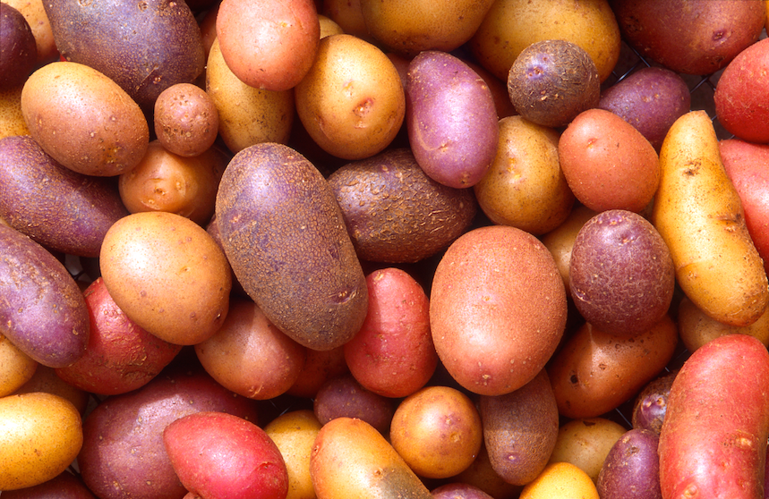
First off, a little history of the dataset. The packed SiO2-sphere dataset was sent to me by Peter Høghøj of Xenocs, as part of a demonstration dataset measured on their Xeuss SAXS instrument. Since the SiO2 spheres are packed in a random dense system (Figure 0), the volume fraction is going to be about 0.634 [1].
1: A quick run with SASfit
Peter mentioned he could get a reasonable fit using SASfit, with a model of Gaussian distributed spheres and a structure factor consisting of a Percus-Yevick hard-sphere (HS) interaction model assuming the local monodisperse approximation (LMA). Trying this, I got the fit shown in Figure 1, resulting in the size distribution shown in Figure 2 (fit parameters given at the end).

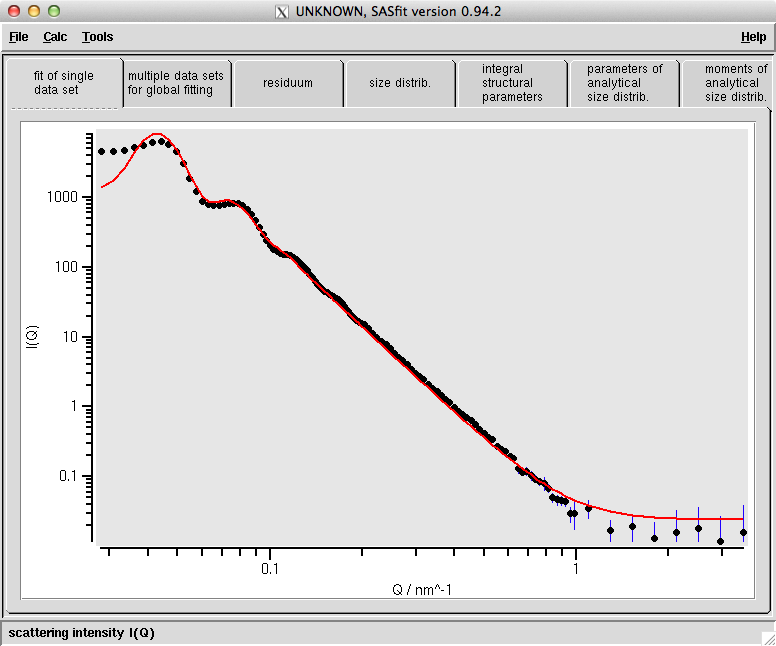
The fit is not bad indeed, with most of the intensity described well apart from the very low-q region. It is worth mentioning at this point that most structure factors are not intended to be used for such very dense systems, as some of the assumptions used in their derivations are no longer valid. Nevertheless, humanity is known for abusing everything, and structure factors are no exception.
2: Adapting McSAS
So far, I haven’t shown anything new. However, previously I claimed that McSAS also had a model for dense spheres using the LMA. This would then be a perfect dataset to put it to the test.
First results were horrible, and the method did not want to converge at all. Suitably discouraged, I left it for a week or two, with that nagging feeling of unfinished business piling up.
After a while, the nag became too much so I took a second look at the implementation, comparing my implementation of the HS model with the one used in SASfit. There were two problems.
One of the exponents in the equations was supposed to be four, not two. That was surprising, as I checked and rechecked the equation when I implemented it. Long story short, it looks like a typo may have slipped into some of the HS descriptions in the papers of J. S. Pedersen [2, 3]. However, there is a clear description of the HS derivation by Kinning and Thomas [4].
The second problem was really one of my understanding in implementation, resulting in that infernal factor of two discrepancy cropping up again (the radius to be used for the HS interaction description was supposed to be two times the particle radius). Anyway, once understood, this was quickly solved.
3: Applying McSAS to the data
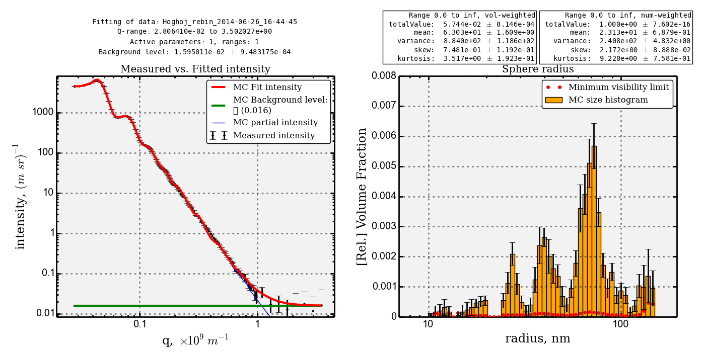
So now we have a working Monte Carlo model, and we can test how well it works. The data uncertainty is (very) low, and the LMA dense spheres model is quite slow. Therefore I have allowed the volume fraction of the interactions of the contributions to vary between 0.6 and 0.64, which speeds up the process quite a bit. The result is shown in Figure 3. It fits to within the uncertainty of the data.

This fit shows a size distribution consisting of a main feature, but also appears to show a minor feature. If so inclined, we can use this information to adapt our SASfit fit by adding a second distribution. Beware of the increased instability of having too many fit parameters, however! A second note is that the LMA might not be perfectly applicable in this dense system, and it could be that this inapplicability results in additional compensatory features in the size distribution.
Nevertheless, this is a result I’m quite happy with (for obvious reasons). But this fit also means we can play a bit more and investigate how this result really depends on the assumptions. For example, I have stated in other work that the result of dense systems is dependent on the choice of structure factor parameters, but is this really the case? Let’s find out.
4: Variability with volume fraction
[ed: In order for me to finish this blog post in a reasonable time, I’m going to relax the convergence criterion a little, which will result in slightly poorer fits and larger uncertainties, but you don’t mind, do you?]
It turns out I cannot get a good fit with the volume fraction below 0.5, so that’s a bit of good news. I can do it with a volume fraction of 0.5, however, and the resulting size distribution is very different to that we obtained before (Figure 4). We can see a lot of peaks appearing at smaller sizes, and the population parameters are now quite different. So we know that we can drastically affect the shape of the size distribution found in SAXS if we are 20% off from the correct volume fraction!
So can we go in the other direction? If we consider we have perfect (HCP/FCC) packing (never in your randomly-packed life!), we would have a volume fraction of 0.74. Well, that one doesn’t quite fit easily but we can just fit a volume fraction of 0.72. The result in Figure 5 shows this, it is now clear that we can let the little side-bump at around 50 nm in the original size distribution to disappear by going to higher volume fractions!

So we can get a wide range of size distributions simply by tuning the volume fraction. It therefore looks like the volume fraction has to be known quite accurately when analysing the data, and that it cannot be a fit parameter alongside the distribution.
4.1: A little more in detail
We thus found out that we can change the size distribution we are getting by selecting a different volume fraction. This is a good example that data ambiguity is the core problem of SAXS and this issue is highlighted in modern form-free fitting methods. Classical methods put strict requirements on the shape of the size distribution which therefore limits the volume fraction to a single solution.
So without providing external information you cannot make an unambiguous judgment on which is the most likely distribution. We can input information based on physical considerations, which say that random packed material has a volume fraction of about 0.62. In this case, there is only one solution. Ideally, though, you would like to verify the volume fraction in another way, perhaps through use of the X-ray absorption factor of the sample combined with the exact dimensions of the sample cell (this is where sandwich-type cells work much better than capillaries). Yet another way would be to measure the density of the sample using a densitometer.
However, we have also found that we cannot go too far. So we can use this procedure to find a coarse measure of the volume fraction and the size distribution either by manually trying volume fractions, or by letting the volume fraction vary freely (Figure 6). It won’t be accurate, as evident from the error bars, but it will give you a measure. And some idea of what it should be is sometimes a useful result in itself!
5: Conclusion:
This is of course just a quick play through the data analysis with dense structures. I’m satisfied with the way the model and the fitting is working, and I am happy to be right that the structure factor parameters strongly influence the resulting size distribution. It shows that we need extra information in case of ambiguity from theoretical considerations or from other techniques. There appear to be very few shortcuts in SAS data analysis!
6: One more thing:
There is one last thing I have not mentioned: resolution. In this case, instrumental resolution was provided with the data, but not used. The smearing resulting from this may affect the data analysis as well. It is certainly something that can broaden the resulting size distribution or even prevent the fit from working at all (not shown here), especially for (near) monodisperse samples. We need to work on implementing this in the MC method, to find out what its effect would be. It may happen, let’s see what happens in due time…
7: Acknowledgments:
Thanks to Peter Høghøj at Xenocs for sending me the interesting data and allowing me to talk about it freely.
8: References
[1] C. Song, P. Wang, H. A. Makse, A phase diagram for jammed matter, Nature 453 (2008), 629–632
[2] J. S. Pedersen, Analysis of small-angle scattering data from colloids and polymer solutions: modeling and least-squares fitting, Adv. Colloid and Interf. Sci. 70 (1997), 171–210
[3] J. S. Pedersen, Determination of size distributions from small-angle scattering data for systems with effective hard-sphere interactions, J. Appl. Cryst. 27 (1994), 595–608
[4] D. J. Kinning and E. L. Thomas, Hard-sphere interactions between spherical domains in diblock copolymers, Macromolecules 17 (1984), 1712–1718
9: SASfit fit parameters:
Sphere * Gaussian dist: N=4.6e-8 (fit), s=11.4 (fit), X0=75.0 (fit) * LMA hard sphere Structure Factor: fp 0.62 (fit) + Flat Background: c0 = 0.024 (fit). Reduced chi-square: 156.2
Leave a Reply