
This has been a very interesting last couple of days. I was unable to join Zoë Schnepp and Martin Hollamby for our SAXS beamtime at Diamond. Instead, I decided to try and join in from abroad. The plans were ambitious: to do on-the-fly high-quality data correction and analysis. In the end there we achieved partial success.
[NB: I am still a bit sleep-deprived, so please forgive the potential incoherence of this post.]
[NB2: A bit more digital ink has been spilled on this topic by Martin and Zoë as well.]
As explained in my previous post, I had been preparing for two weeks to upgrade and customize the data correction procedures to handle the data automatically. Data files could be dumped in a monitored directory on the server, from where they would be picked up, picked apart and spliced with other data. Finally the data is corrected using the imp2 data correction procedures, which I have been working on for the last year.
This was tested using test datafiles sent to me by Andrew Smith from i22. Fortunately, data correction could be done on one of the beamline desktop workstations. Naturally, test datafiles can only get you so far for preparation, and automation was not possible for mask- and background file generation, so I was ready to handle the first measurements when the beamtime started (See Figure 0).

Communication with Zoë and Martin was established using Twitter in particular, which proved to be a reliable tool if a bit limited (140 characters, you see. Though this may also have enforced brevity). Skype was only used twice, but it remained tough to understand one another without dedicated microphones for this at the beamline. Longer messages and some data passing could be done using e-mail. The real data transfer tasks were done using rsync, though we were severely hindered by the relatively large files, and the incredibly slow internet connection in Japan (the fastest domestic plan we could get is practically still many times slower than our European connectivity six years ago, even though on paper they should have been quite comparable.).
There were some minor issues in the data analysis. Firstly, the monitor readings were time-dependent, and needed normalisation. Secondly, the monitor readout was scaled with an order of magnitude that only appeared in the “description” of the detector in the datafiles. Since the autoscaler could not be reliably switched off (resets of the detector systems would switch it back on), this information needed to be picked out of the description and taken into account as well.
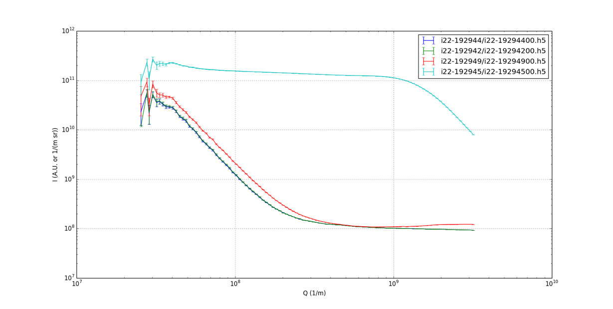
Then there was an issue with connectivity. It turns out that the Japanese domestic connection was a bit too slow to pass on the corrected data within a reasonable timeframe. This made it tough to look at the data once corrected, in particular for the “real” measurements. The real measurements were done on 21 points along the capillary, measuring 10 images per point (to avoid overloading the Pilatus detector counters). Datafiles for such measurements weigh in at about 250MB per file.
After a rather long-ish beamline preparation (troubles due to freshly restarted synchrotron and recent fixes at i22), it was time for me to get to work. After processing and setting the mask and background files (Figure 1), we were just about to start running normal measurmeents (this was Saturday morning for me, around 9 AM) when disaster struck. An item was left on the motorized optical table where it shouldn’t have been, and ran into the flight tube when the table was moved up. Cue dislodged motors on the table. Calling it a night (for them) allowed them to sleep a bit, and me to screw around a bit fixing my mountainbike (reparing damage from another, unrelated crash).
That evening at 9 PM my time (I am about 8 hours ahead of them), they reported imminent resumption of work, with about 20h remaining in the beamtime. Deciding against ASAXS for the moment, it was time to run normal SAXS. To prevent too many issues with absorption, the energy was set nice and high. It took me a while to set up the background and mask files again (being suitably groggy), only to find out about the monitor count issue, and having to fix, redo and redo.

A one-letter typo in my code also delayed me a bit, but in the end, data corrections were running smoothly, chugging away at anything that was thrown at it and spitting out quite excellent data.
We even measured some sample containing a partically crystalline material. Having the proper background subtraction and correction procedures in place (though a Lorentz correction needs to be applied before analysis of crystalline data), means that this is probably one of the few WAXS measurements with proper background subtraction and realistic data uncertainty estimates! I expect angry diffractionists to stomp down my door for saying that anytime now. But to be honest, the typical background subtraction procedure in WAXS data processing leaves a lot to be desired (estimating a baseline by eye, not taking transmission factor into account, etc…).
Automated data fitting was a bit more tricky. Though some data fit quite well, most of the data has features which were not (yet) readily described using a simple Monte Carlo model. It looks like we still have some way to go before we can do this part without intervention at the beamline.
So for me, this tele-beamtime felt like a real beamtime: hardly any sleep, crashes at the beamline and groggy coding sessions. However, it also was the first SAXS beamtime where we walked away with already quite-well corrected data (some things such as monitor drift are still to be checked and perhaps re-processed for that). That made it possible to check the corrections and adjust the measurements accordingly during the beamtime. Which is so much better than finding out you missed something several weeks afterwards. Very much worth repeating.
Would I rather be at home or at the beamline? Well, the issues with internet speed meant that much of the graphical feedback could not be done which would have helped. For that alone, it would have been better to be at the beamline. At the home office, however, I did have a 1 minute travel time to bed and a fresh supply of really good food (thanks to a supporting family), so that has big benefits too. I guess we will find out what I will do when the next beamtime comes along!
Leave a Reply