

Estimating uncertainties on data values has always been an important and under-emphasized part of small-angle scattering. Uncertainties are critical to your data: they tell you what is most likely a real difference, and what is probably just measurement noise. Fortunately, many datasets come complete with data uncertainties, but there are still quite a few cases where this is not the case, or where the provided uncertainty estimates are unrealistic. So what can we do?
The uncertainties are often imagined as the random point-to-point differences between neighbouring datapoints. While gradual differences can also be considered part of the uncertainties, they are often not random and therefore should be corrected for.
So far, I have estimated uncertainties in a variety of ways, one of which is done during the azimuthal averaging of data (making the 2D dataset a 1D dataset). It considers the variance between datapoint values in a single integration bin as an estimator. While this works well, it does require that you do the integration yourself. This is not always an option, for example when collecting beamline data, or when using manufacturer-supplied data reduction software. Perhaps there is another way.
What we would like to estimate is the difference between a datapoint’s expected value and the actual value. One method of doing this is to consider (e.g.) five neighbouring datapoints, fit a linear relation between them, and use the difference between the linear fit and the actual value as an estimator. While it can work, and is a method I considered using, it does seem to be a bit of an arbitrary method (there is no reason why five neighbouring datapoints should be linearly correlated, for example).
We can perhaps arrive at a different solution (hinted at in the title) by considering the properties of data noise: it is a high-frequency component of the data. In other words, noise randomly oscillates rapidly from one datapoint to the next. If we want to get an idea of the magnitude of this high-frequency component, maybe we can do bandpass-filtering of the data to extract just that.
[ed: There is a big disclaimer here: this is an idea I came up with over the week-end. It may not work, it may not be appropriate, and it has probably already been investigated 30 years ago. This blog post is here trying to find out if it could maybe work, or if it is impossible to get reasonable information out.]
The easiest way to do bandpass filtering is to use Fourier transforms. With the Fourier transform, we move from data-space to frequency-space, turning our data from individual points to a superposition of waves. Sounds complicated, but it is rather easy to move from data-space to Fourier-space and vice versa in any math software such as Python.
One side-note to keep in mind is that the discrete (fast) Fourier transform we are using assumes periodic boundaries of the signal, i.e. it assumes infinite side-by-side copies of the data. This is no problem, except that one side of our data is very high, the other side low. Stitch two copies together side-by-side, and you get a very abrupt change and therefore a big feature in the frequency spectrum. One solution for this is to attach a mirrored version of the data so that the joins become less jarring.
So here is a quick example moving a real dataset in Python from data-space to frequency space. Note that we are completely ignoring Q-spacing: (Comments preceded by “#”):
# load our data:
dval = pandas.read_csv('Data.csv', delimiter=';').values
# split into Q, intensity and uncertainty:
Q = dval[:,0]
I = dval[:,1]
E = dval[:,2]
# because FFT likes periodicity without steps
DoubleI = np.concatenate((I[::-1],I))
# move intensity to frequency space:
FI = fft.rfft(DoubleI)
# and back to data space:
NewI = fft.irfft(FI)
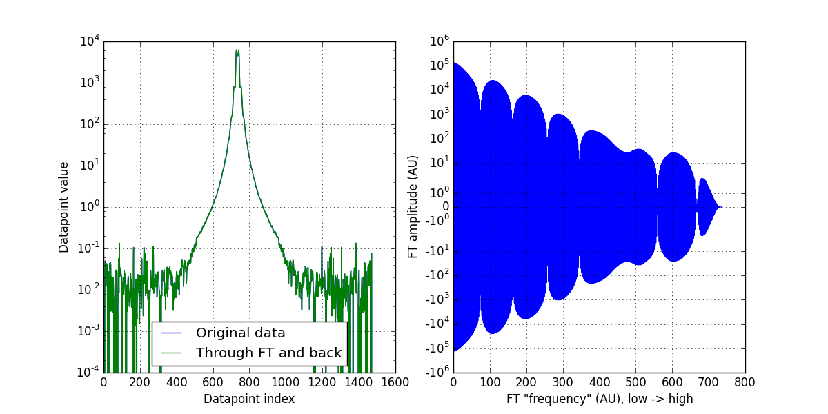
Easy, right? FI is the data representation in frequency-space (complex numbers signifying amplitude and phase), and I is the data as we are familiar with. I show the double intensity and the Fourier components in Figure 0. There does still seem to be something artefact-y going on (indicated by the seven-ish regular dips). but I am not overly concerned with that now. An inverse FT returns exactly our intensity as it was.
Bandpass filtering is the removal of frequency components. A low-pass filter lets low frequency components through (slow data variations), and removes high-frequency components. A high-pass filter lets high frequency components through, and removes the gradual changes.
When we move our data to frequency-space, we can apply such filters. Our FI data has the low frequencies at the beginning of the array, and the high frequencies at the end of the array (note: this is the case since we used a symmetrical FFT which only works for data in real space. Check if this is the case for the FFT you are using). By reducing the values at either end of the array, we can filter low or high frequencies (or anything in between).
Whenever you create a filter window to multiply your Fourier components with, always be careful to avoid sharp edges (sharp edges and Fourier transforms don’t mix very well). So I use a “normal” distribution’s cumulative distribution function to be a smooth-ish step function of my window:
# load distributions:
from scipy import stats
HWindow = stats.norm.cdf(range(size(FI)), loc = size(FI)-500, scale = 80)
# Normalise distribution to 1
HWindow /= HWindow.max()
# and get the inverse window as well:
LWindow = 1 - HWindow
We apply the filter by element-wise multiplication with the frequency components of the data:
# inverse real FFT on the windowed data:
HI = fft.irfft( FI * HWindow ) # High-pass
LI = fft.irfft( FI * LWindow ) # Low-pass

And we are done! We have now two new datasets, one containing the high frequencies, and the other containing the low-frequency data. We see that the low-pass filtered data (cyan curve, RHS of figure 1) is a bit of a smoothened version of the original data (see below), and the high-pass filtered data is the very high-frequency component in our data.
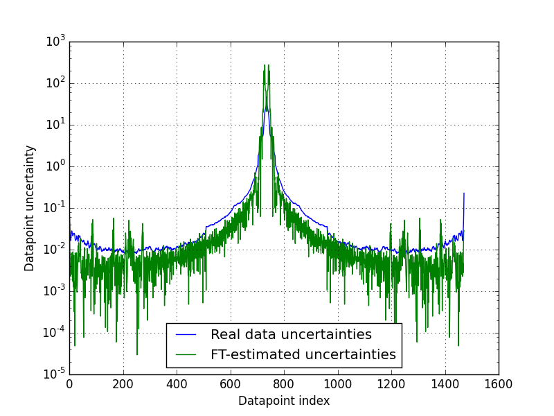
When we compare the uncertainties we get this way with the uncertainty estimates that were provided with the data, we see that they match a bit (Figure 2).
Did I cheat? Yes I did cheat a bit. See the numbers used for the filter window (location and scale in particular)? I played around with them until I got a reasonable result. A bit more thought will be needed to discover how we can determine these values without human input… OK, maybe a lot more thought.
But it looks like we can use this method to do some filtering, and maybe get an idea about the noise in the system. I’d put this in the “maybe” column of ideas.
Another question that is sometimes posed is: “can we use this to smoothen our data” (i.e. use the low-pass filtered datacurve)? The short answer: yes you can, but you really shouldn’t! Modifying data this way can change the intensity profile of the data, and risks removing real features as well.
Interestingly, we can use Fourier transforms as well to play around with smearing functions from imperfect experimental set-ups. More on this another time.
Appendix: Full code example.
import pandas
# load our data:
dval = pandas.read_csv('Data.csv', delimiter=';').values
# split into Q, intensity and uncertainty:
Q = dval[:,0]
I = dval[:,1]
E = dval[:,2]
# because FFT likes periodicity without steps
DoubleI = np.concatenate((I[::-1],I))
# move intensity to frequency space:
FI = fft.rfft(DoubleI)
# and back to data space:
NewI = fft.irfft(FI)
# Figure showing the data and back figure(figsize=[12,6]) subplot(121) yscale('log') xscale('linear') grid('on') plot(DoubleI, label = 'Original data') plot(NewI, label = 'Through FT and back') xlabel('Datapoint index') ylabel('Datapoint value') legend(loc=0)subplot(122) yscale('symlog') xscale('linear') grid('on') plot(real(FI), label = 'FT amplitude') xlabel('FT "frequency" (AU), low -> high') ylabel('FT amplitude (AU)') savefig('Data_and_FT.png')# Filter: # load distributions: from scipy import stats HWindow = stats.norm.cdf(range(size(FI)), loc = size(FI)-500, scale = 80) # Normalise distribution to 1 HWindow /= HWindow.max() # and get the inverse window as well: LWindow = 1 - HWindow# IRFFT: HI = fft.irfft( FI * HWindow ) LI = fft.irfft( FI * LWindow )# Show result # show filters on top of Fourier spectrum: figure(figsize=[12,6]) subplot(1,2,1) yscale('symlog') plot((real(FI)), label = 'FT amplitude', color = 'k', lw = 2) plot(LWindow, label = 'Low-pass window', color = 'cyan', lw=4) plot(HWindow, label = 'High-pass window', color = 'red', lw=4) ylim([-5e-1, 2e5]) xlim([0, 735]) xlabel('FT "frequency" (AU), low -> high') ylabel('FT amplitude (AU)') legend(loc = 0) grid('on')subplot(1,2,2) yscale('log') xscale('linear') grid('on') plot(DoubleI, label = 'Original data', color = 'k', lw = 1) plot(LI, label = 'Low-pass filtered', color = 'cyan', lw = 1) plot(HI, label = 'High-pass filtered', color = 'red', lw = 1) ylim([5e-4, 1e4]) xlabel('Datapoint index') ylabel('Datapoint value') legend(loc=0)savefig('FT_window_and_filtered_I.png')# Show final error estimates: figure() DoubleE = np.concatenate((E[::-1],E)) plot(DoubleE, label = 'Real data uncertainties') plot(abs(HI), label = 'FT-estimated uncertainties') legend(loc=0) yscale('log') grid('on') xlabel('Datapoint index') ylabel('Datapoint uncertainty') savefig('FT_uncertainty_and_real_uncertainty.png')
Leave a Reply