Why we never may be able to get a calibration curve: a matter of coherence

2015-02-17 Brian Pauw Blog posts 9

For years, we have been trying to compare scattering patterns from different instruments. While this leads to reasonable results, there are precious few cases of true agreement despite the focus on data corrections (one example of agreement: [0]). My guess: we have not been considering coherence in these comparisons.

Coherence is essential to all forms of scattering and diffraction, not just for coherent diffraction imaging and other fancy techniques. We have coherence when the electromagnetic waves in a particular area are in phase. All diffraction and scattering effects consider interference effects of these in-phase waves before and after their interaction with matter in the sample.

All school experiments with double slits and diffraction gratings all assume coherence in the incoming waves to arrive at the observed effect. For areas where the radiation is not in phase, the effects of matter on the different waves do not form constructive and destructive interference, and will not form consistent off-angle wavefronts. As such, they will not add to the nanostructurally related information we are trying to obtain (but can add to an incoherent background contribution).

For typical small-angle experiments, the radiation in our sample area is in phase in some places, and out of phase in other places. The sample volume is therefore filled with small regions of in-phase radiation, so-called “coherence volumes”. These volumes are internally coherent, but the different volumes are not in phase with each other.

Therefore, when we do a scattering or diffraction experiment, we get diffraction and scattering from each of these coherence volumes. Each of the intensities (but not the phase) from these coherence volumes can be summed to obtain our scattering or diffraction pattern [1].

The longitudinal size of the coherence volumes is defined by the monochromaticity: the better the monochromaticity, the longer the waves stay in phase along the beam direction. The transversal size $\zeta$ is the one we are typically interested in in scattering experiments. This is defined by the collimation and instrument geometry. It can be estimated as $\zeta = \lambda l / w$ , where $\lambda$ is the wavelength of the radiation, $l$ the distance between the beam-defining collimator and the sample, and $w$ the size of the collimator opening [2].

Laboratory instruments, such as NIMS’ Bruker Nanostar, typically have quite small transversal coherence lengths. In our prior experiments, we estimated this to be on the order of 200 nm [3]. In those experiments, we also saw a noted absence of scattering from big, high contrast scatterers (observed in electron microscopy) whose sizes were well beyond this estimate.

(note, however, that this coherence length is quite a bit larger than the distinguishable nanostructural dimensions imposed by the q-limits of the instrument itself. In the aforementioned experiment, we were limited in our quantification of the size distribution of nanostructural objects up to several tens of nm. Objects larger than this limit will typically contribute only their “porod”-slope, somewhere around $I \propto q^{-4}$ . In the analysis of scattering patterns, the presence of such a sloped background only indicates that there are large scatterers present, but we cannot say how large as they fall beyond the determinable range imposed by the q-limits.)

Synchrotron instruments, on the other hand, can have much larger transversal coherence lengths, so that much larger structures will also contribute to the scattering pattern. At Diamond’s I22 beamline, for example, the beam defining slit is about 19m from the sample, with typical dimensions of 2.04 x 1.3 mm (H x V) at a wavelength of 0.1 nm [4]. This means that the transversal coherence length is approximately 930 x 1460 nm (H x V) [5]. One interesting sidenote is that one may therefore see small differences in vertical and horizontal scattering patterns for very polydisperse samples. This means that the scattering pattern from the synchrotron will look different than the one obtained in the laboratory.

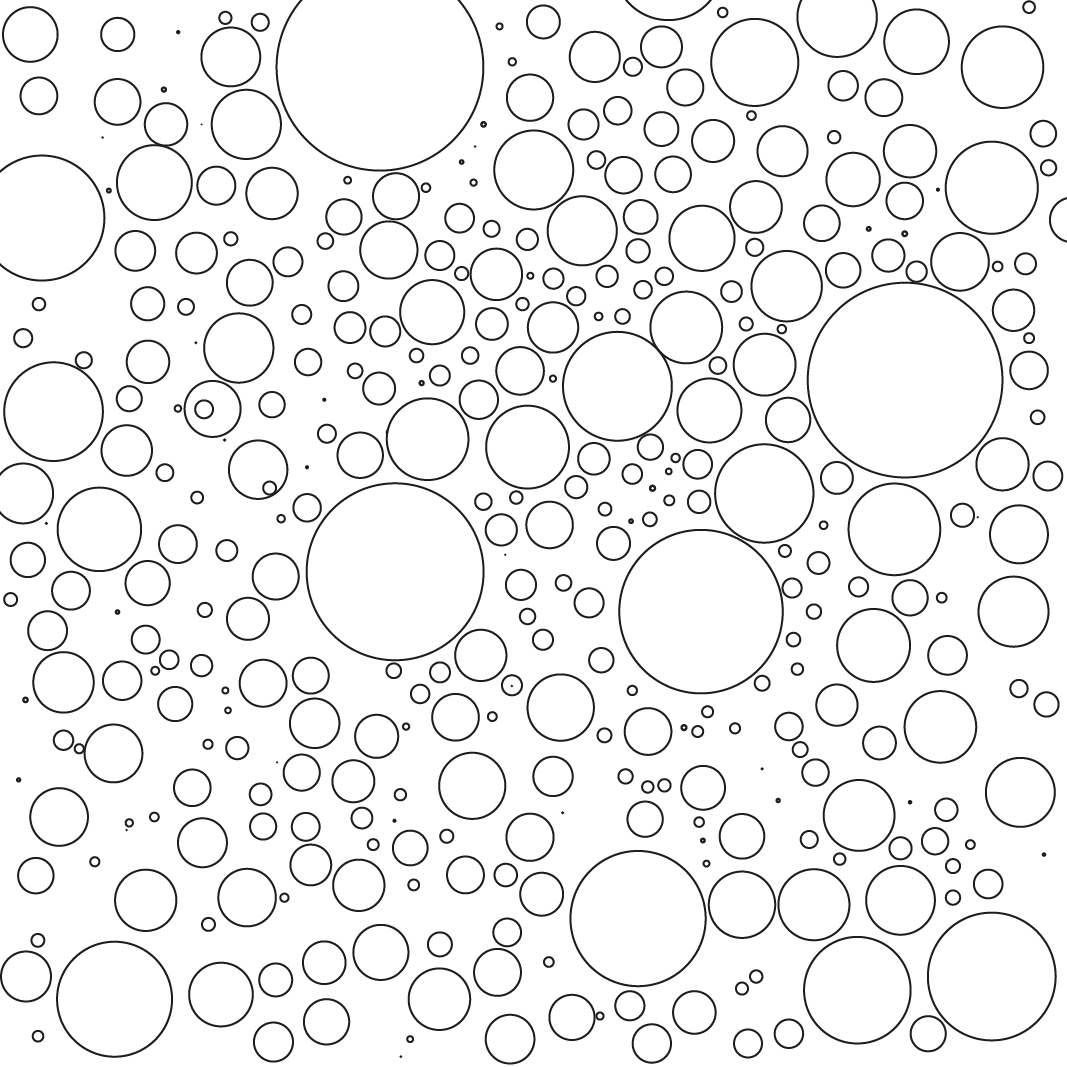
To explain graphically, I have created a field with polydisperse spherical objects (Figure 1). This serves as my two-dimensional sample cross-section.

**Figure 2:** Small coherence volumes over our sample from Figure 1, with the scatterers removed that are not enveloped by the coherence volumes.

If I have a laboratory instrument, I will have some (more or less randomly placed) small coherence volumes in this sample. Superimposed, these are shown in Figure 2, where I removed the scatterers not enveloped by a coherence volume.

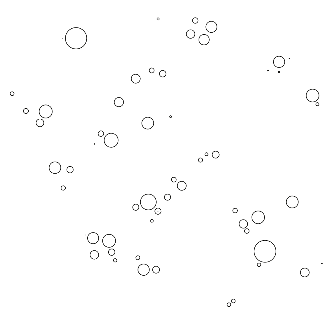
**Figure 3:** The scatterers enveloped by the small coherence volumes

The scatterers enveloped are shown in Figure 3. It can be seen that they are limited to a rather small-ish subset of scatterers.

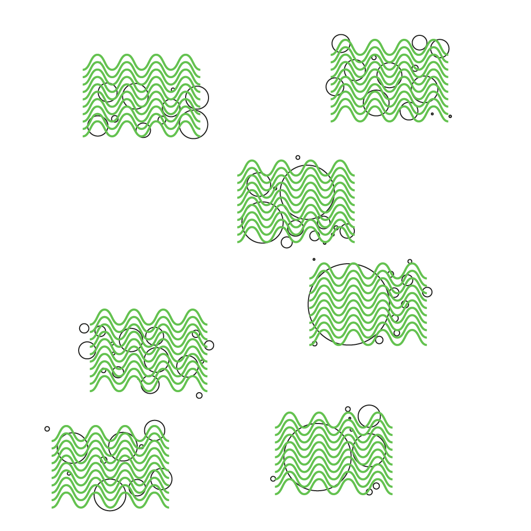
**Figure 4:** Large coherence volumes superimposed on scatterers in our sample. Scatterers outside the coherence volume have been removed.

Contrast this with larger coherence volumes and the scatterers they envelop (figs. 4 and 5). These now contain a significant (surface) fraction of large scatterers which will contribute their sloped behaviour to the scattering pattern.

**Figure 5:** The scatterers enveloped in the big scattering volumes.

To try and visualise the effects on a scattering pattern, I fired up SASFit to give me a simulated pattern for a gaussian distribution of spherical scatterers [S1], superimposed on a uniform distribution of large objects. Assuming a maximum estimated coherence of either 800 or 1600 nm, we get the patterns shown in Figure 6 (using settings S2 or S3, respectively).

**Figure 6:** Difference in scattering pattern for a coherence length limit of 800 vs. 1600 nm.

So yes, there should be a big difference in the scattering patterns based on our quick estimation of coherence. Of note is that the information we are interested in, the small gaussian distribution, is less visible for our virtual instrument with a larger coherence length. So perhaps it would be nice to be able to tune our coherence (by changing our collimation settings), so we can physically remove the information of scatterers we are not interested in, and increase the signal of the scatterers we are interested in.

However, it also shows that — if this was our calibration material –, we would still get different scattering patterns from different instruments. This means that intercomparisons of scattering patterns may be incorrect. However, the nanostructural information that the scattering patterns contain should be similar. So we can compare the real-space results of calibrants obtained from a variety of instruments instead.

Bonus question: calculate the horizontal and vertical coherence of a Kratky instrument, and of converted diffractometers such as the Rigaku Smartlab or Panalytical X-pert.

References:

[0] A. R. Rennie et al. Learning about SANS instruments and data reduction from round robin measurements on samples of polystyrene latex. J. Appl. Cryst. 46: 1289–1297, 2013. http://dx.doi.org/10.1107/S0021889813019468

[1] F. v. d. Veen and F. Pfeiffer. Coherent x-ray scattering. J. Phys.-Condens. Mat., 16:5003–5030, 2004.

[2] B. R. Pauw. Everything saxs: small-angle scattering pattern collection and correction. J. Phys.: Condens. Matter, 25:383201, 2013.

[3] J. M. Rosalie and B. R. Pauw. Form-free size distributions from complementary stereological tem/saxs on precipitates in a mg–zn alloy. Acta Materialia, 66:150–162, 2014. arXiv:1210.5366.

[4] Andrew Smith, I22 senior support scientist, personal communication (e-mail 2015-02-16)

[5] The beam is slightly focused, so I do not quite know how the coherence length is affected by this focusing. This is a quick estimation, YMMV.

SASFit settings:

Q limits: 0.01 – 1, number of datapoints N = 49.

[S1]: gaussian distribution of spherical scatterers: N=5e3, s=10, X0 = 20.

[S2]: S1 + Uniform distribution of spherical scatterers: N=0.5, Xmin = 100, Xmax = 800.

[S3]: S1 + Uniform distribution of spherical scatterers: N=1, Xmin = 100, Xmax = 1600.

Fred
2015-02-17 at 17:59

Very interesting thoughts, Brian ! You are right that these aspects are usually completely overlooked !

However I think your approach to quantify it is much too sketchy:
– The coherence volumes are not randomly placed spheres, with nothing in between. The coherence length is a measure of the gradual loss of spatial coherence. The further you go from one position, the less phase relationship you got with that position. Strictly speaking, you still have a phase relationship between two separated objects but it vanishes with distance
– I think you can not simply remove the “larger” objects from your simulations. If the object is larger than the coherence volume, what you probe of it is the coherence volume, you are not simply disregarding that object. In other terms, the limiting size that you can probe is the image of the source…

Thanks for sharing.
Fred
Brian Pauw
2015-02-19 at 08:49

Hi Fred,

Thanks for your comment!
Indeed, the coherence volumes are not strictly bound, but I had trouble drawing that in illustrator :). The gradual loss of coherence could probably be modeled as a convolution with a gaussian (or $\sin^2$ ?) function. Also, the estimator I gave is only a rough estimator, I think I just found another such estimator in another paper, but differing by a factor $\pi$ .

As for the larger object, the larger the object, the higher the chance that the coherence volumes will only probe a single phase (in the object), as opposed to probing the interface. If it probes a single phase, there should be no scattering.

I have also no idea if you get scattering at all if a coherence volume envelops just one phase interface (e.g. top half phase one, sharp interface, bottom half phase 2). Time for me to try Fourier transforming a sharp interface function!

I would very much like to explore this topic further, and am very interested in finding out what people think about it.
Fred
2015-02-19 at 20:34

it sure does produce scattering… Think of it as the product of the microstructure and the coherence volume. The resulting scattering is the convolution of the microstructure signal and the coherence signal (e.g. Transform of the source)
Brian Pauw
2015-02-20 at 08:47

So that would imply that (given a suitable instrumental set-up) the coherence can be analyzed or characterized through the scattering of a straight edge… Hang on, didn’t I read a paper about that? (to be continued…)
Adrian Rennie
2015-02-20 at 17:29

Brian,

You raise some interesting questions about scattering. I suspect that for most purposes of small-angle scattering the discussion of resolution (smearing as described by dQ/Q, Q is momentum transfer) and ‘coherence’ result in the same approximations. There are, of course, some experiments such as correlation spectroscopy, phase contrast, etc. where particular attention to coherence is needed. Here are some thoughts that are not very profound.

In general a measurement of intensity at a particular momentum transfer will depend on resolution: this is easily seen in the neighbourhood of sharp maxima and minima. Different instruments and configurations of instruments can give substantially different ‘results’. This is seen in the data in the round-robin paper that you cite as reference [0]. The different reported values do not imply that some are right and others are wrong as long as there is an adequate description of the resolution. One must be careful: simple scaling of data so that intensity approximately matches in a limited range of momentum transfer is not adequate if the effects of resolution are significant. Even comparison of data from different configurations of the same camera needs attention to resolution. This is a common mistake in simplistic data reduction.

As might be expected, the SANS community have often used poorer resolution and it is becoming more common to find some information in neutron data that can be used in modelling. The SAXS community have often ignored resolution except for slit cameras (e.g. Kratky) or Bonse-Hart geometry. However a number of measurements with pin hole cameras do need attention to resolution. The focussing elements are often quite different in horizontal and vertical directions as combinations of monochromator crystals and mirrors are used. For I21 at Diamond we had to estimate some values for divergence for the data shown in reference [0]. The ageing of the mirror can be a significant uncertainty in how it performs. Since the paper was published there is now some other data from ESRF, MAX-Lab and the Australian Synchrotron on the same material and, as might be expected, resolution effects are significant. The assumption that an approximation of perfect resolution does not introduce a significant systematic error in analysis needs to be addressed in quite a number of experiments.

If one is seeking standards or secondary standards for intensity calibration, there is a preference for ‘flat scattering’ samples with small dependence of intensity on resolution. This comes with the unfortunate disadvantage that they will usually be weak scattering samples!

Apart from these simplistic practical comments, I am not certain that the calculations based on coherence volume are straightforward. Your analogy with light can help provide explanation. Even the intersection of a coherent wave front with a single sharp edge can give rise to ‘diffraction’. This is often demonstrated with an expanded laser beam impinging on the edge of a razor blade. One does not need to envelop an object within a coherent beam to observe scattering. I think that the same argument will apply to SAXS. Some care is needed in doing precise calculations with large objects. Even with X-rays the effects of refraction may be significant. The case of partial coherence or distribution of coherence of the wave and distributions of polydisperse objects needs attention. Provided the system is dilute the average of scattered intensity can be calculated but once the system is concentrated the interference factor (or structure factor) relating to correlations needs to be estimated as well as the validity of any decoupling approximation for the effect of polydispersity.
Adrian Rennie
2015-02-20 at 17:40

As regards calibrating scattering instruments, a single straight edge may be difficult for normal SAXS instruments but 20 years ago we used pin holes (made for elecron microscopy) to verify the performance of a low angle light scattering instrument:

R. H. Tromp, A. R. Rennie R. A. L. Jones Kinetics of the Simultaneous Phase Separation and Gelation in Solutions of Dextran and Gelatin. Macromolecules 28, (1995), 4129-4138.

DOI: 10.1021/ma00116a012

In the experiment we used scattering from a circular aperture to verify the lack of distortion from optical components and to check the intensity which is well-known from the Airy function.
Brian Pauw
2015-02-21 at 10:00

Thanks for all the good comments, Adrian!

I see gratings being used in literature to check for coherence as well, but I have only seen examples of this in reflection. The pinholes may be a nice idea to try as well.

I think that the concepts of resolution and coherence are similar, but not quite the same. The coherence is a property defined only by the source, the collimation and the sample position. The resolution, on the other hand, also needs to take detector aspects into account. We can have excellent coherence, but terrible resolution (for example if we have a detector with big pixels). Note that the coherence estimates I get for our lab instrument and the synchrotron are typically an order of magnitude larger than the resolution (maximum distinguishable object size) of the instrument.

However, my emphasis is that even though we are not doing anything special with it (coherent diffraction, imaging, or suchlike), we still may need to take it into account when considering regular small-angle scattering (see the estimated effect of coherence on the simulated scattering patterns). The intensity we detect at low Q can contain either a large or small contribution from very large scatterers, depending on the degree of coherence.

As for the desmearing, or taking resolution into account, I very much like the paper by Norbert Stribeck (doi: 10.1107/S0021889808015021), in which he desmears two-dimensional scattering patterns from the same instrument in different configurations to arrive at a complete, well-overlapping pattern. I still don’t really grasp the implementation details of the desmearing, however, so I have not been able to do the same…

I agree that considering coherence, however, is not going to be as simple as the blog post appears to indicate. This is also mentioned by Fred in his comments. Perhaps I need to put a disclaimer at the top emphasising that it is only a rough approximation to highlight that we may need to take coherence into account to better understand normal experiments.

Thanks again for the good discussions!