

Time for another short investigation into data corrections? Good. Let’s take a quick look at the linearity of our Bruker HiStar detector.
What are we doing
We are testing here whether our detector gives us a proportional (linear) response for high countrates as it does for low countrates. At a certain level, most detectors will “choke” on the high number of photons coming in, rejecting photon signals due to a variety of effects. We will be testing this for our HiStar detector: a 2D, gas-filled wire array detector.
Bruker themselves indicate that the detector is supposed to be highly linear, quoting reasonable countrates (also for their later detectors). A closer look, however, reveals that Bruker considers any deviation up to 10% (!) to be within linearity [0]. That, of course, will not be sufficiently accurate if we are supposed to be having data with an uncertainty better than 99% (note that this is a personal goal, not based on any metrics).
There are two main types of detection nonlinearity that can occur, Either global nonlinearity due to too many photons per second impinging on the entire detector surface, or a local nonlinearity due to per-pixel overloading. We will check both.
For this test, I have been using two samples of glassy carbon, one thin, one thick, to be my main source of scattering. The thin GC sample is the standard sample from Jan Ilavsky that we use for our absolute intensity calibrations. A combination of GC thin (1 mm), GC thick (3 mm), and GC thin & thick (1 & 3 mm) can then give me a signal on the detector with varying count rates.
Setup
This combination of samples has been measured for 300s at six different settings for generator current (50, 40, 30, 20, 10 and 5 mA, all with 50kV voltage. we use a Bruker Nanostar SAXS instrument with a high-speed molybdenum rotating anode source). Theoretically, the ratio of intensities for the three samples should be the same for all generator settings. We will check this by checking the intensity in a few locations (ROIs) on the detector images.
It should be noted at this point that the Bruker software already applies a deadtime correction to the detector images, which is supposed to correct for this effect even before we get to touch the images. However, as shown in [1], the minimum uncertainty estimate on the datapoints should then deviate. So we will check if we can see something in the evolution of the uncertainties as well.
Total Countrate Results
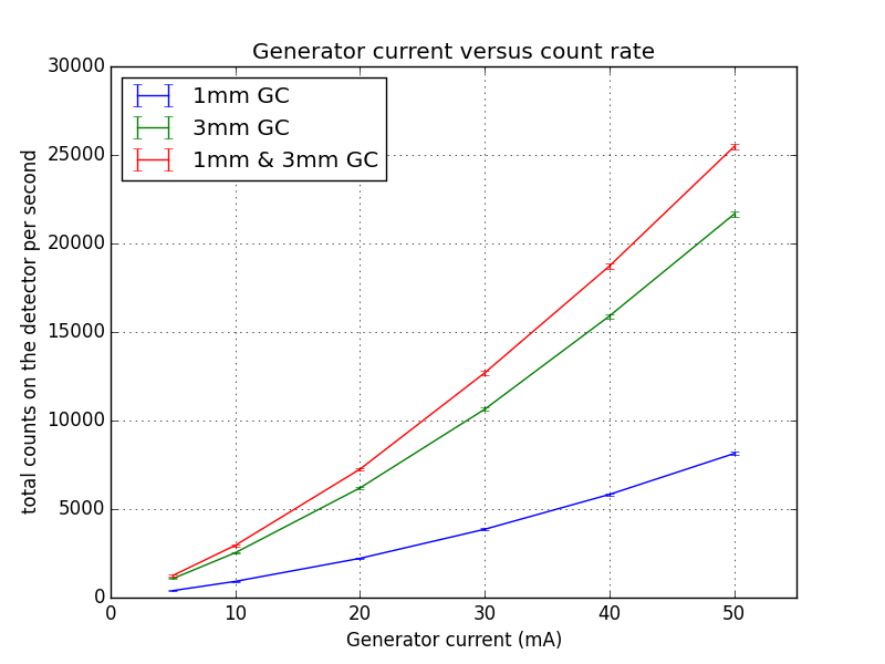
First, we can look at the total detector countrates. When we plot the number of counts detected versus the generator setting, we see that the countrate does not appear to be linearly dependent on the generator current (Figure 1). While it is theoretically supposed to be, there are a number of reasons why it shouldn’t have to be in practice. These include different heat loads on the target and optics at different currents, imprecise current measurements, etc.
This is the reason I measured three different sample combinations. For each setting, the ratio of intensities between the samples should be the same, and ideally also independent of the countrate.
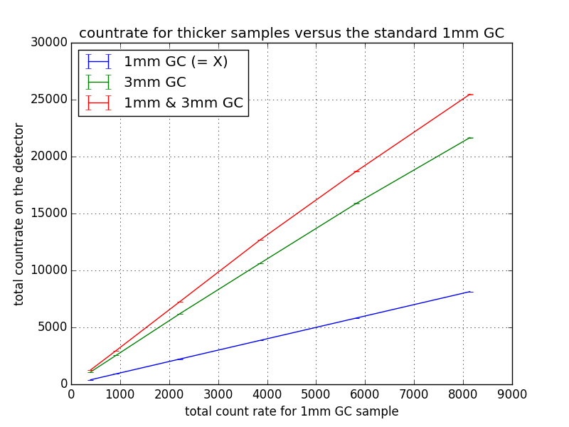
Therefore, taking the 1mm GC sample as the “calibrated” countrate (on the X-axis), I can plot the sample set again. From this, we can already see that the total countrate of the three samples is not quite linear (Figure 2). Normalizing by the counts for the 1mm sample (to obtain the intensity ratio), we see what appears to be systematic deviations of the total number of collected counts for the 3mm and 1 & 3mm samples (Figure 3).
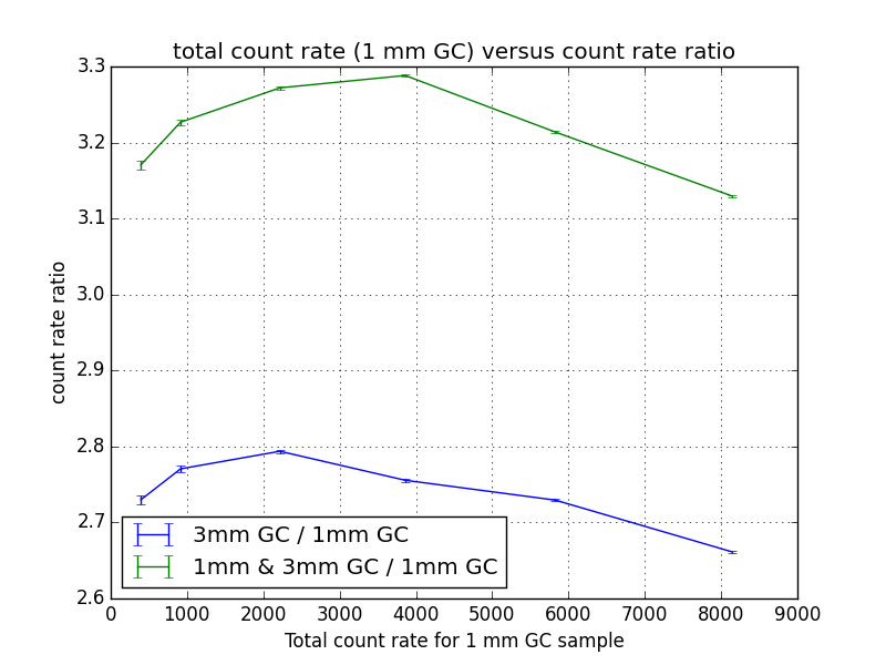
These curves are looking a bit curious, with a maximum at about 2000-4000 cps, after which a gradual decline in the count rate ratio can be observed. For the latter measurements, this means that we are detecting fewer counts than we should be for those thicker samples. It also shows that the deadtime correction implemented by Bruker does not fully compensate for the loss in detection capacity at these rates. Note, however, that all deviations remain within 10%. Therefore it is “linear”, according to the Bruker definition.
The initial bump can have two explanations. It is either an artefact of Bruker’s deadtime correction, or (more worryingly), it might mean that the count rates of our reference sample (1mm GC) are already exceeding the count rate limit!
This would make me slightly unhappy as we typically use the 1mm GC sample for our calibration measurements. That would imply that my absolute intensity calibrations could be slightly off.
As for the local linearity checks, I will need to take a raincheck on that. I have the data (which you are more than welcome to have a play with), but this article is becoming too long already, and my time is running out for today.
See you next week!
[0]: Vantec 2000 spec sheet (upgraded, but basically similar detector as the Bruker HiStar). Downloaded here, March 17, 2015.
[1]: D. Laundy and S. Collins. Counting statistics of x-ray detectors at high counting rates. J. Synchrotron Rad., 10:214–218, 2003.
Hi Brian,
I would highlight the fact that, because you are working with a gas detector (a system that counts single events instead of an integral sum of events), the non-linearity you are now talking about comes from dead-times effects, i.e. the fact that two events must be separated by a minimum time to be discriminated. CCDs and solid state detectors can be non-linear for other reasons.
In other words, checking non-linearity is important for all detection systems, but its correction is different for each system, and is quite easily done for gas detectors.
After identifying that non-linearity is attributable to dead-time(s) comes the questions of paralysability: if an event is missed because it comes too quickly after a properly recorded event, does it prolong the dead time or not?
If the electronics allows to save events not only with their coordinate but also their time, one can reconstruct an histogram of these events (number of events versus delay between events). This should be a single exponential decay, as the scattering process should be Poissonian. In case of a non-paralysable dead-time, the exponential decay will have a clear cut-off for short delays (there will be zero event for delays less than the dead time). In case of a paralysable dead-time (each non-detected event increases the dead-time), the histogram will have not only a cut off for short delays, but also a cut-off for high number of events. A fit by a single exponential decay for longer delays will give the “true” count-rate.
The interesting point is that, by recording X,Y,t instead of only X,Y, one could properly correct for dead-times effects without actually knowing the dead-time. Given that dead-times are due to several factors (gas ionisation, charge detection, ADC, memory buffer, synchronization between events on different wires), it can be useful to actually check the exponential decrease of this histogram, instead of assuming a constant dead-time.
It also allows to check that the electronics does its job properly, as one can identify events that should not exist, or events that are missing.
We did that on V4, the SANS at HZB, which has a multi-tube (Reuter-Stokes) 3He detector and an electronic with 100 ns time-stamping. Beyond the fact that the dead-time was slightly different for different tubes, we also saw that the electronic had several (minor) issues, associating occasionally wrong spatial or temporal addresses to detected events; firmware updates and software treatment could then be used to correct that.
Hi Sylvain,
Good point, I should have mentioned (like I did in the review paper) that only photon-counting detectors can be “easily” corrected for with the dead-time model. Other systems such as CCDs or image plates need their nonlinearities checked as well, but those systems will follow different correction models.
As far as I know, the standard Bruker detector does not allow X,Y,t-output of events (at least not available to users). This, then, is something for which it may be interesting to build some new electronics (Raspberry Pi- or Arduino-driven, hopefully). There is another, undiscussed problem that can occur with multiple near-simultaneous photon-events on the wire-detectors, which is that a photon might be counted in a completely different location. You will see this for very high countrates, sometimes as stripes or echos of features. These countrates are well beyond what should be used, however.
What you discuss about the detector paralysing is also considered in the model by Laundy (see reference 1). If I remember correct, they indicated that this should not affect the correction.
My first concern is to find an easy way of characterising such nonlinearities. The GC option seems to work for flooding the detector, but the local countrates are still very low. I do not expect to see much local overloading (though I haven’t gotten around to that yet). For that I may need a crystalline sample to give me a nice locally overloaded signal.