Ultra-SAXS on powders: pow(d)er to the people!

After the imminent move, “my” instrument will become unavailable again (it cannot travel with me). That means that now is the only time available to get at least some data out of the instrument. So how far did we get since the previous measurements?

First off, most of the planned upgrades worked, but the improved detector (Amptek XR-100SDD in combination with a XIA digital pulse processor) did not. That meant that I had to revert the detector to the previous scintillation-type detector. This is mostly alright, but (even with a rather narrow energy window) that detector has a “dark” countrate of 0.12 cps, which complicates measurements at high Q.

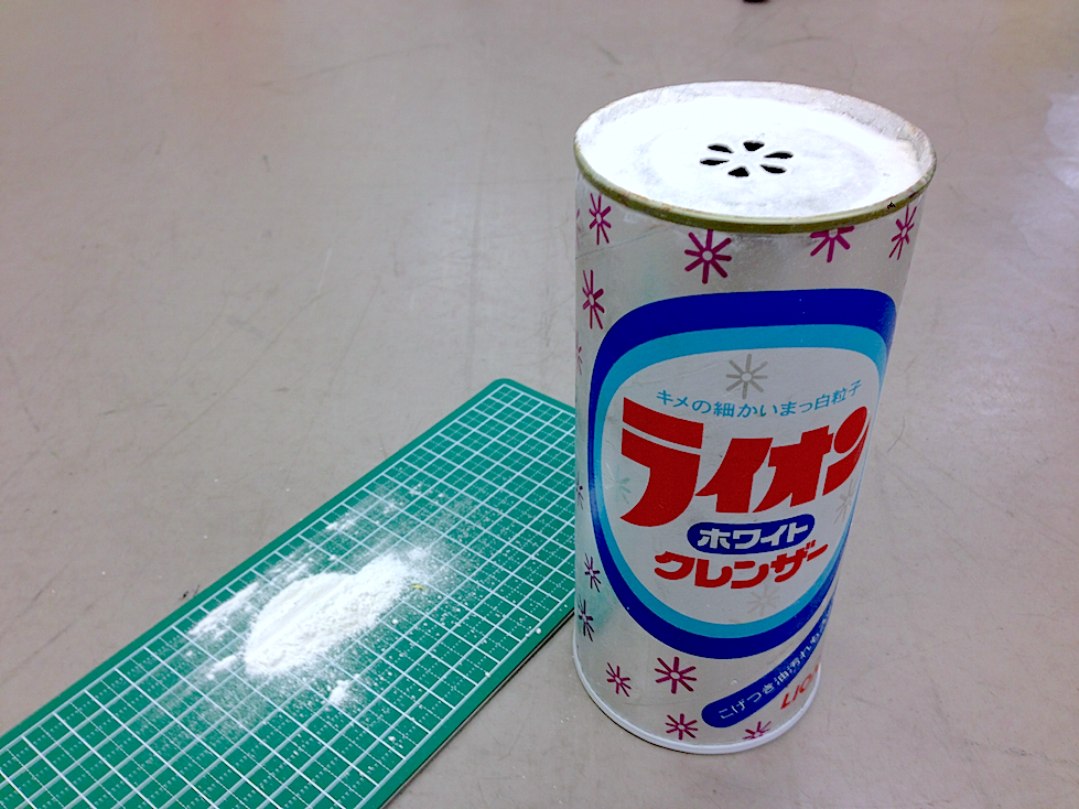
So we need strongly scattering systems to get some results off. Powders rank amongst the top in scattering power, so the first thing we tried was the only powder sample in the lab: scrubbing powder (Figure 1). Loading this into a ~1mm thick holder, we found significant absorption but also a humongous scattering signal (Figure 1).

The pattern shows that the powder consists of large particles, perhaps around the micrometer regime. It also shows the powder does not contain much smaller components: the flanks adhere nicely to the behaviour, which we would expect for smooth surface scattering of the larger particles. Pete Jemian mentions that the lack of an “unscattered beam”-signal indicates multiple scattering is going to be a major issue for this measurement. Obviously, we needed to improve some of the scan parameters, and (perhaps) switch to a more metrologically interesting sample.

I was very happy to receive just the right sample from Yojiro Oba: He provided some “Hypresica” silica nanoparticles of size 0.2 µm and 1 µm. These were packed into 2mm thick, plate-like sample holders (printed from plastic), and measured. Based on our previous findings, we increased the number of measurement points, and increased the measurement time at high angles.

Each measurement consisted of ten scan repetitions (to assess stability and verify the measurement uncertainty), with each scan lasting about 12 hours. Each scan consisted of 320 points, unevenly spaced to sample the full Q-range with a higher density at low Q than at high Q. Measurement times per point were 60 seconds, except for the outer 80 points, which were measured 200 seconds each.

The results are very interesting. There remains quite some absorption (carrying with it the risk of fudging due to multiple scattering effects, in particular for the 1 µm particle sample), but the 200 nm particles show clear oscillations. The 1 micrometer particles do not, however. This could be due to the (unknown) dispersity preventing us from seeing oscillations. Note that the 1 µm sample scatters similar to our scrubbing powder!

The absorption remains (very) high, so I will re-measure these samples using 1 mm sample holders and see if that improves matters. Every measurement takes about four to five days with the current settings, however, meaning that I can only measure five more samples before my time here runs out. However, even at this rate, one could measure 50 to 100 samples in a year with the right planning.

Finally, for all these “slit-smeared” measurements, you need to either: a) de-smear the data, which magnifies the uncertainty and risks introducing fake features (see this post and its comments), or b) smear the model you are trying to fit to the data. While the latter is much safer than the de-smearing procedure, very few fitting programs appear to support this approach (perhaps only SANS analysis programs).

At the moment, I am trying Pete Jemian’s “jldesmear  (git repository)” program for de-smearing of the scattering patterns. Once I have figured that out, expect another post.

So the take-away points from these tests are:

• Yes, you can do Ultra-SAXS on a laboratory instrument, even with a microfocus source, and even at molybdenum k-edge energies (actually, that turns out to be quite a nice energy). All you need is time and a strongly scattering sample. (Though a better detector would be a great help!)
• For the best benefit, however, this should be combined with an excellent SAXS machine. An excellent SAXS machine should be able to provide accurate, verified measurements up to a q resolution of (note that this means the instrument’s theoretical resolution should be (much) better than that). Such a limit should provide decent overlap with USAXS data up to .
• Powders are suitable samples for these instruments, but pay attention to the transmission, and keep an eye out for the multiple-scattering effects!