

[Quick note: I am also giving a talk at ESRF next week, on the 3rd of December, in the Science Building Seminar Room 035 at 15:00]
Two of you have informed me of amazing work published last week. You may remember that we briefly mentioned 3D SAXS a while ago here, of which a more detailed write-up is still to follow. The added information content in a full 3D scattering pattern should be quite interesting, and would allow f.ex. the testing of the MC method in three dimensions, as opposed to the two demonstrated here.
Now the ante has been upped by two (somewhat related) groups, having combined 3D scattering pattern reconstruction with computed tomography. This gives you spatially resolved three-dimensional scattering patterns, i.e. a 3D scattering pattern for each three-dimensional voxel in space.
The papers are the following:
- Marianne Liebi et al.: “Nanostructure surveys of macroscopic specimens by small-angle scattering tensor tomography” [who was also the winner of the SAS2015 Kratky Prize]
- Florian Schaff et al.: “Six-dimensional real and reciprocal space small-angle X-ray scattering tomography” [note that Marianne Liebi also co-authored this paper]
In the same issue, a “news & views” article can be found by Peter Fratzl, who previously also worked on 3D pattern reconstruction. This article adds some more context and a more gentle introduction to their findings.

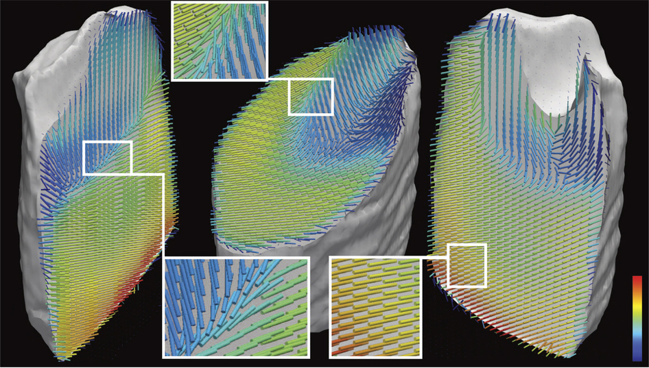
The approaches of the two groups differ slightly, with the Liebi work using spherical harmonics to describe the 3D scattering patterns, whereas Schaff did not. In my non-expert view, the use of spherical harmonics may be more resilient to reconstruction artifacts appearing in the scattering patterns, but I may be wrong about this.
Both groups managed to calculate their solutions on more-or-less commercially available computer systems, making this approach more achievable by normal laboratories. Total reconstruction times were reported to be on the order of a week. Both groups used biological samples, which, as indicated in the SI of Schaff, may suffer from radiation damage in these long experiments (40h for Schaff, 36 h for Liebi). In fact, it is hard to think of samples that would not be damaged by such exposures. Bonus points to the group of Schaff for using Kieffer & co.’s pyFAI for their initial azimuthal averaging, surely helping enormously in the reduction of the scale of the optimization problem.
The obtained data looks amazing from both, and the technique is set to add much value for (not-so-nondestructive) nanostructural investigations of many hierarchical materials. With this, we may finally have a good use for those newfangled bright synchrotron sources!
Leave a Reply