Scattering from arbitrary objects, part 1: proof of concept

“How would [X] scatter” is a question asked by many, and already answered by a few. To calculate the scattering of arbitrary objects, there are a few things we can do…

There are a variety of methods available to calculate scattering from structures. To name but a few, there is a nice method by S. Hansen [1], or one can use a numerical Fourier transformation (as I also did during my Ph.D), for example using the method by K. Schmidt-Rohr [2]. However, these all require that you define your shape in “their” language, and since I’m the stupid kind of lazy*, I don’t want to do that.

Having played for a bit with open source 3D drawing packages for our 3D printer, it is clear that these have been painstakingly tuned so that one can draw efficiently. Most of those programs spit out a STereoLithography (STL) file, which describes arbitrary shapes by defining their surface (and only their surface) as collections of connected triangles. Would we perhaps be able to use those to define our input shapes? All we need then is a method to turn a 3D surface into a scattering pattern.

Starting out by barking up the wrong tree, I tried to determine the chord-length distribution function (CLD) from our surface definition. I got the random points on the surface, and could calculate the CLD and the intensity, the latter in a bit circumlocutious way. However, it turns out there are three different definitions for the CLD [3], and mine was not quite adhering to any of them. This meant that it worked for spheres, but not so much for elongated objects due to the non-homogeneous density of chord angles.

W. Gille and S. Hansen advised to use the pair-distance distribution function (PDDF) instead. Both the CLD and the PDDF indicate a distribution of lengths between pairs of points, however the CLD requires the points to be on the interface of the object, while the PDDF has the points distributed throughout the volume of the object.

According to [1], this can be translated to a scattering signal through:

and
, with that last p(r) being our PDDF.

The move to the PDDF implied a bit of a hassle: the only Python library that could turn an STL surface definition into a volume object is the VTK library. This is a beast of a thing, and difficult to install. In the end, I had to install Anaconda Python on my notebook (alongside the other Python flavours) which has a precompiled VTK package. A little elbow grease later, and I had that working well. However, VTK implies Python 2 and QT4, both of which are getting a bit old in the teeth.

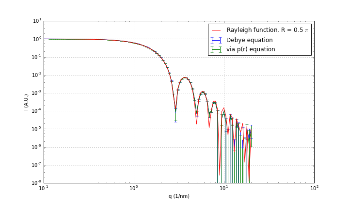
Using many tips from this site when it came to picking points and placing them inside STL objects, a PDDF calculator was quickly programmed. It is reasonably fast, managing to find 1000 points inside the object in several seconds, but it does occasionally add an obviously outside point to the list. I hope that ends up in the numerical noise.

These points can be used to calculate the scattering pattern in two separate ways: either through the PDDF, or directly using the Debye equation for points. As always, we calculate the uncertainty on the scattering pattern by repeating the procedure a number of times, and calculating the mean and the standard error of the mean.

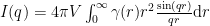
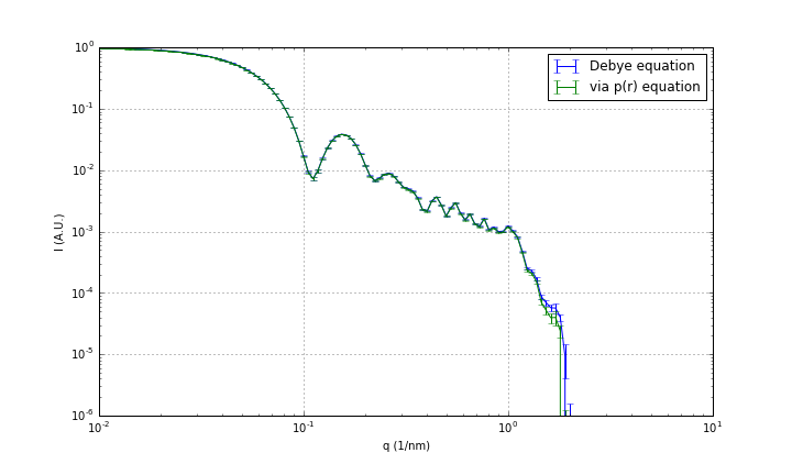
The first and most common check is to test the method against a sphere. That one’s easy, and shown in Figure 1. Unfortunately, there seems to be a factor of discrepancy between my values and the Rayleigh scattering function, and so one of my next tasks is to figure out where that bug lies. The other bug is the aforementioned occasional point lying outside the object, as shown in Figure 2.

However, the agreement between the determination of the scattering pattern via the direct Debye function, and via the PDDF is quite remarkable. My initial suspicion was that the method via PDDF would result in data with a much higher accuracy, but that is not supported by the data.

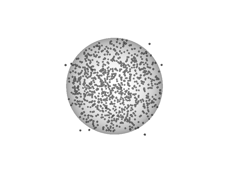
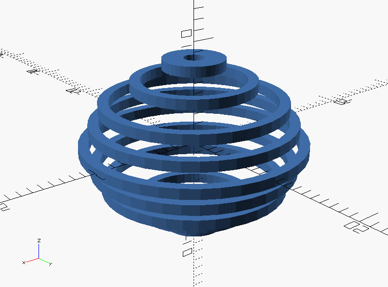
Just to show you other interesting patterns, Figure 3 shows the pattern from an elongated ellipsoid, which works much better than a sphere due to the absence of low dips. Lastly, there is a pattern from rings in close proximity (Figure 4). Doesn’t that remind you of certain stripy features (Figure 5)?

Ok, so with my tongue out of my cheek, there is still some work to be done. There are at least two known bugs to resolve, and there is some validation to be done once those have been ironed out. There is a further limitation in that the information at high values drops off dramatically (due to the low probability of having points in very, very close proximity). However, this seems like a nice approach, and is certainly worth pursuing.

I hope I can present you with a “Part 2” within a reasonable time. As usual comments can be deposited in the box below!

*) The stupid kind of laziness is where you find yourself spending a lot of time figuring out how you’re going to avoid the tedious task (often by programming something really smart). The time spent, however, is typically much larger than the actual time saved. On the plus side, it’s a good (fun) way to keep active, and you do stumble across things that will help you in the future, so I don’t mind this kind of laziness.

[1] S. Hansen. Calculation of small-angle scattering profiles using monte carlo simulation. J. Appl. Cryst., 23:344—-346, 1990.

[2] K. Schmidt-Rohr. Simulation of small-angle scattering curves by numerical fourier transformation. J. Appl. Cryst., 40:16–25, 2007.

[3] W. Gille. Chord length distributions and small-angle scattering. Eur. Phys. J. B, 17:371–383, 2000.