

The displaced volume correction (pointed at here and here) is one that, to my great regret, does not appear in the “Everything SAXS” paper as I did not know about it at the time. However, it is time for some further thougts on it. We start with its definition…
This is a correction that only needs to be considered for measurements on samples or sample dispersions, where the sample takes up a significant fraction of the volume. A rule of thumb would be to use this for samples which occupy a volume fraction of at least 1% within the dispersant *.
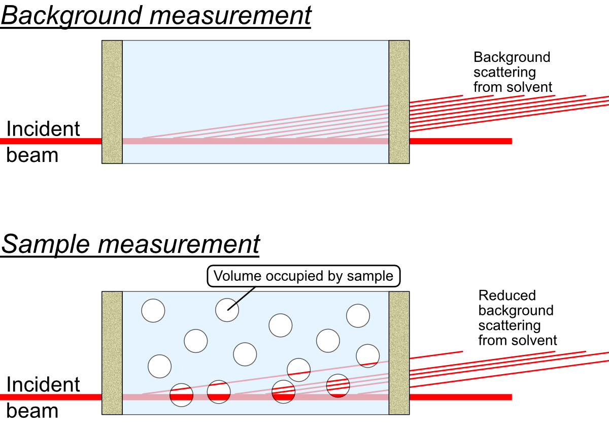
What happens in these cases is that there is a reduction in the amount of background material that the primary beam passes through, since a part of that space is now not occupied by background material but by sample instead. There is simply less background material in the beam. This implies that there is a reduction in the background signal, by an amount proportional to the volume of sample in the beam. This is not something that is compensated for by the transmission measurement: the sample may have a very similar absorption probability as the background, but still occupy a large fraction of the space.
What complicates matters firstly is that this only reduces the background signal originating from the solvent, while leaving the background signal from the sample container walls unaffected. This means that the background signal needs to be “disassembled” into its components, and that the background scattering signal from the liquid needs to be reduced in a scaling procedure.
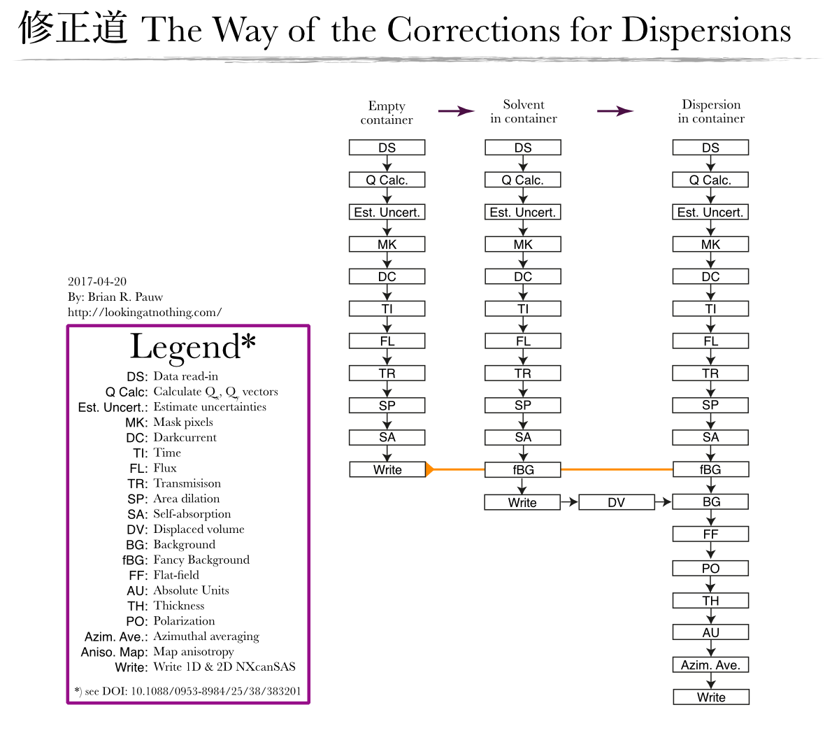
What you do, see figure 2, is to use the “fancy background subtraction” procedure to separate the wall scattering from the solvent scattering. You use the same procedure to separate the wall signal from the dispersion scattering. The solvent scattering can then be multiplied with its (remaining) volume fraction, and subsequently subtracted from the dispersion scattering with a simple background subtraction procedure, to obtain the scattering pattern from the sample only.
The second complication is that there is a bit of a chicken-and-egg problem: you cannot do this correction without knowledge on the volume fraction occupied by the sample. That volume fraction, however, may result from the scattering pattern analysis of the corrected scattering pattern (which you don’t have yet). It may be possible to do this correction in an iterative manner (yet untested). Alternatively, the volume fraction of analyte needs to be determined in another way.
So will it matter? To be honest, I am not sure I ever had a case when this played a large role, but if we are to achieve the ultimate precision, this is to be taken into account. Its effects must be significant if 1) the analyte volume fraction is significant, and 2) the scattering signal from the sample is weak vs. the signal from the solvent. Proteins in solution are a prime example, but also dispersed polymers and vesicles may be affected by it.
*) While this holds for a range of samples, here we’ll consider the case of an analyte dispersed in a solvent.
Brian, you say that the displaced volume correction cannot be compensated by measuring transmission. I disagree with this. If one measures the flux transmitted by the sample in cell and empty cell respectively and corrects the raw intensities accordingly, there is no need to apply the displaced volume correction.
On the other hand, if one calculates transmissions by using tabulated values for the lineic absorption coefficient, then you are right, we ought to have this extra correction.
Hello Oana,
This is not a correction for a cell with and without liquid, but for a liquid with and without a voluminous sample.
We can do a Gedankenexperiment: Imagine we have a strongly scattering solvent, like cyclohexane (the signal from that itself is really quite impressive). We put this in a sample cell that doesn’t scatter or absorb, which holds 1 mm of our cyclohexane solvent in the beam. We measure a signal of 10 counts per second from this cyclohexane at a given angle. So far so good.
We put into this solvent a sample of plastic spheres, which have the exact same linear absorption coefficient as cyclohexane. We put so many of these spheres in that they take up a volume fraction of 0.25 in the solvent. We still have a total of 1 mm of spheres in cyclohexane in the beam, and the x-ray absorption is exactly the same as for the pure solvent. However, we will see only 7.5 counts per second from the cyclohexane, since there is only 75% of it in the beam. That means that if you want to isolate the sphere scattering signal, you should subtract only 75% of the signal you got from your 1mm of pure cyclohexane.
So this correction is unrelated to the transmission factor correction.
Hi Brian,
In my opinion, if the spheres and the solvent have the same linear absorption coefficient, there is no electronic contrast and consequently no scattering. So I don’t think it is a good example.
If you otherwise measure the transmitted intensity of a solvent (=> Isolvent) and of a mixture 25% spheres + 75% solvent, the contribution of the solvent to the latter will be 0.75 * Isolvent only.
So in my opinion if you accurately measure the transmitted intensity and correct the raw data accordingly, you do not need the excluded volume correction.
The example would work. The scattering in case of the solvent comes from density fluctuations in the solvent. If my spheres have a contrast of zero vs. the solvent, but a super uniform density, you will see a reduction in the scattering signal by 25%. There is then less material in the beam with the density fluctuations.
I can also modify my example to clarify: I have a layered particle with dense and not dense layers. These particles have the same *overall* transmission factor as the solvent. You will not measure a difference in transmission factor, but you will have to reduce Isolvent to 0.75 before subtraction in order to isolate the particle scattering.
In neither of these cases will an accurate transmission measurement show you any difference between solvent and sample.