Detectors for good SAXS

A few questions have come up via the blog asking what kind of detector would be helpful for getting good SAXS measurements. Having worked with a few different types, perhaps I can shed some light on what has worked for me and what hasn’t, ending with some hopes and wishes for the future.

If you are not familiar with the basic detector types and their properties, skip to below first to read a small summary on detectors. Otherwise, here’s the deal:

What do we need?

For SAXS, we need highly accurate measurements over a very wide dynamic range. These need to be corrected, in particular, we need to subtract a second, highly accurate measurement. These measurements ideally consist of counted photons.

On photons…

The photon is not only the smallest unit of scattering intensity we can measure, it is also the only one. Whereas integrating detectors measure an unknown amount of intensity, when we are counting photons, we have a few benefits. Firstly, we can be sure we are measuring the smallest amount of scattering we can measure, there is no increase in sensitivity that would aid us here. Secondly, we get an uncertainty estimate for free in the form of the Poisson statistics. These stochastic counting statistics give us the smallest possible uncertainty on a scattering intensity value. It can be larger, but never smaller than this. So whatever detector we get, photon counting ability is pretty high on the wish-list.

Hybrid pixel detectors and wire chambers are two detectors that count photons. Wire chambers, however, are limited by their dynamic range and position sensitivity, and need to be corrected for image distortions as well. Localized high intensities can easily desensitize the wires at that area, and (at less high intensity) create ghosts or copies in the image. So we need dynamic range.

On dynamic range…

When we are measuring SAXS patterns, we are spanning many orders of magnitude in scattering intensity. For some samples this can be as much as four decades in intensity per decade in Q (or three decades if you are working with slit-smeared detectors). With modern instruments, we can span several decades in Q, and so we usually span much more than four decades in total, maybe six or seven.

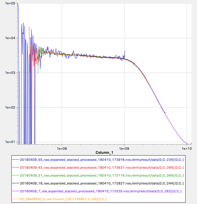
We can even go one step further: it is surprisingly useful to be able to measure the direct beam as well on the detector. We can use this to get decent estimates on the transmission factor, and on the primary beam photon flux. These two bits of information are not only indispensable for proper data correction, but also allow you to go to absolute intensity without any effort (and fully traceable). Calibration with water at a specific temperature, Lupolen or the NIST SRM3600 glassy carbon is no longer necessary. We have demonstrated this in our MAUS recently, with our traceable intensity within 3.5% of the certified SRM3600 values (see Figure 1), after a nice set of our modular data corrections (many of which are now implemented in DAWN).

As you know from our USAXS experiments, the primary beam intensity can be many orders of magnitude larger still than our scattering signal, perhaps another three or five orders, so now we’re talking dynamic ranges of ten orders of magnitude. This can go one of two ways: up in maximum countrate, or down in background countrate.

The maximum countrate is set by the detector electronics: the speed of the peaking amplifier and the peak shape analyser circuitry in particular, and also the ability for the detecting element to recharge or reset after a detection event. There are not many detectors that can measure a photon stream of higher than, say, photons per pixel per second, but our dream SAXS detector would have to go much, much higher than this: Diamond’s i22 beamline, for example, has primary beam fluxes approaching photons per second. Although these are not all concentrated on one pixel, they aren’t spread over that many. Secondly, a detector material that is stable under this high energy load is also hard to find. So, going up is hard.

The other way is down. While we can’t increase any sensitivity down there — we are counting photons after all — we can do another thing: filtering out some background. For synchrotrons, this doesn’t always make a lot of sense. Their high beam and scattering intensities lead to short exposure time and less sensitivity to some background contributions such as cosmic- or natural background radiation. For lab sources, however, we are much more sensitive to these backgrounds as our primary beam intensity is much more limited. You cannot just “subtract” backgrounds either: the uncertainties add!

Background can be reduced by smart instrument design, in particular by keeping materials out of the beam. This includes kapton windows and air paths, flight tube windows as well as helium, which should be kept out of SAXS machines if at all possible. Additionally, the signal from a sample container should be minimized (through smart container choices), and edge scattering from pinholes or slits should likewise be removed.

Another unwanted background is the signal from natural background radiation and cosmic rays, as well as scattering signals from impure X-ray sources. The latter appear in many SAXS machines to some extent, even those with multilayer optics: low-energy X-rays are passed through by specular reflection off the multilayer optics, higher order energies from brehmsstrahling are reflected by multilayer optics as well as some single crystal monochromatisation methods. Apropos, nickel-filtered copper radiation is much more “dirty”. So we need to be able to select the energy of the photons that we want to see, so we can cut away the low-energy photons as well as the high-energy photons, leaving a small energy channel in the middle that we are interested in.

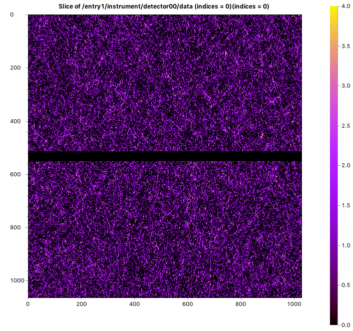
You might consider this to be a small effect. For fun, I measured 12h of these cosmic rays and natural background radiation on our detector. The result is shown in Figure 2. On average, we get about photons per pixel per second. Which doesn’t sound like a lot, but over the entire detector surface, that makes about 14 photons per second. That is the background we are currently limited by, and defines the limit to our dynamic range. This limit could be moved much more through energy filtering.

On energy filtering…

Currently, most hybrid pixel detectors are equipped with one energy threshold in the detection chain. That means we have one step filter, which can filter out lower energy contamination, or fluorescence effects from iron (although this is only possible when measuring with a molybdenum X-ray source, whose energy, 17 keV, is far enough for effective filtering of the 7 keV fluorescence photons). However, we are not able to filter out the high-energy cosmic rays (yet), as a second threshold is only becoming available in detectors now. With that, we could, perhaps, increase our dynamic range by another order of magnitude or two in the lab.

The energy thresholds implemented on these hybrid pixel detectors are also quite broad. Sharper energy thresholds, ideally in the range of hundreds of eV only, would allow us better separation between wanted and unwanted signals, and may even allow us to remove iron fluorescence from a SAXS pattern recorded with a copper source.

On 3D pixel shapes

In two dimensions, the pixels on a hybrid pixel detector are nice: sharply bound within their active area of about 100 square microns with no cross-talk between them. In three dimensions, however, we suddenly get a brick-shaped active detection volume, and suddenly things are not so clear-cut anymore.

Imagine a photon coming in at an angle on a stack of bricks. If the front layer of the first brick does not absorb the photon (and convert it into a cloud of electrons), the photon travels further and may be converted in the volume of the next one. This gets worse the higher the intensity: our 450 µm thick silicon layer only absorbs 50% of our molybdenum-source photons. Not only have we lost photon detection efficiency, we also lost position resolution at high incident angles.

There are improved detectors available, with different sensor materials, that absorb more higher energy photons within a shorter distance. Their markedly higher price, however, tend to outweigh the benefits for now for the average SAXS lab, but the hope is that their price will come down.

What about those gaps? Smaller pixels?

Questions often arise on the gaps between detector modules: if you have multiple detectors, or a single multi-module detector, there may be an area between the modules which does not detect photons. While initially one might think of methods to remove these gaps from the images, through interpolation or by detector movements, they really are not an issue. When analysing these images, we mask the invalid pixels at and around these gaps, and in doing so they become a non-issue (for SAXS at least). Even for oriented scattering patterns, by careful positioning of the detector modules with respect to the direct beam, little critical information is lost. 2D fitting methods can likewise ignore the gaps through masking.

The second question is that of smaller pixels. Yes, small pixels are nice, get you a very smooth image, and can increase your maximum countrate as the flux is divided over more pixels (which is one of the reasons we chose a detector with small pixels in our laboratory). However, with the limiting factors of a beam of about 200 – 500 µm in diameter, and a 2 mm beamstop around that, we are not going to get much better in Q resolution with smaller pixels. Pixels of about will do fine for now (I know, famous last words).

Speaking of pixels, there was once a detector with hexagonal pixels. These are theoretically much nicer to work with for the circular or point-symmetry patterns we work with. However, as soon as you try to imagine image processing algorithms with hexagonal pixels, you will see the issue. Alas, a beautiful, futuristic solution in search of a problem.

On metadata and the future

So the latest detectors are still not perfect, requiring countrate corrections, flatfields, angle-dependent sensitivity corrections or position uncertainties. In addition, we need detectors with better (more) energy windows and even higher dynamic ranges.

Some of the current issues, however, can be mitigated by knowing more: we can correct the detector output, or better estimate its uncertainties, by knowing more about how the photons were counted and (internally) corrected. Extensive metadata needs to be supplied with every detector image, therefore, that allows us to do this. In particular for (national) laboratories seeking accreditation, a good deal of metadata is needed to demonstrate traceability and good laboratory practices. The current NeXus standard is helping in this respect, allowing a structured deposition of critical metadata alongside the collected detector images.

The arrival of the hybrid pixel detector (when the alternatives consisted of wire chambers, CCD detectors and image plates) allowed us to suddenly work a lot more accurately with our scattering data, necessitating more detailed data corrections and demanding more from our analysis methods. It helped to improve reproducibility and traceability of data, let us estimate uncertainties, and allowed us to get rid of several “handwavy” fudge factors. These hybrid pixel detectors have changed our perspective, and I can’t wait to see what the next generation of detectors will let us do!

 

Appendix:

Basic detectors:

The types I have experience with (so far) include (in no particular order):

• various gas-filled wire chambers (single-wire and wire grids)
• image plate detectors
• CCD detectors (tapered fibre and image-intensifier based)
• Silicon drift detectors
• scintillation tubes
• hybrid pixel detectors (both 1D strip and 2D pixel variants)
• PIN-diodes

Basic detectors 0D:

Of these, the scintillation tubes, PIN-diodes, and silicon drift detector are 0D (point) detectors. You can imagine that trying to capture a 2D scattering pattern by moving the detector around and recording the scattering intensity at each position is much too time-consuming.However, they can be used (for isotropic scatterers) to scan in one direction and collect the 1D scattering pattern, as is sometimes done on diffractometer rigs or USAXS machines, and they have some nice features worth mentioning before we move on to the multi-dimensional detectors. Additionally, many of the benefits and drawbacks to these detectors apply to the others too.

PIN-diodes are incredibly simple detectors, with a high dynamic range of seven or more orders of magnitude in intensity. This means that their output is proportional to an x-ray flux within that range. These are mostly sensitive to higher fluxes found at synchrotrons (even beyond ph/s). Two drawbacks: 1) they are (usually) not photon-counting but integrating, so we need to think a little about estimating the uncertainties. 2) they have a noise floor that makes counting longer pointless. Whereas for photon-counting sensors, you can add multiple images together to get more counts (over a longer time), with these integrating detectors, you will end up adding the noise floor too, gaining little to nothing.

Scintillation counters and silicon-drift detectors, however, are photon-counting. That means we can use Poisson statistics to get a lower limit to our uncertainty estimate: the uncertainty estimate can never be lower than the Poisson uncertainty (but it can be larger). Secondly, these detectors generate a signal that is proportional to the energy of the photon, and so we can filter the photon “peak” by energy. This is an important feature as we can now get rid of cosmic background radiation (very high energy photons), a significant fraction of natural background radiation (natural decay processes occurring around us, which also generate photons), and lower- and higher-energy contamination from our X-ray sources that still pass through our mirrors. The first two may become significant, as we will see later, for laboratory instruments. Silicon drift detectors in particular have very good energy sensitivity, allowing us to carefully select the energy band that we’re interested in. Maximum countrates of such scintillation and silicon drift detectors usually top out at about ph/s for the fastest models.

One additional note on deadtime correction: since these detectors count single events, there are some problems if two photons arrive at the same time or very close to each other (from the detector point of view). In the first case, the two are “detected” as a single photon of double energy, and usually rejected if there is an upper energy threshold. In the second case, the first photon temporarily depletes the detecting element, rendering it unable to detect a next one within a short timeframe. These two effects cause us to detect fewer counts than actually landed on the detector surface. The good thing is that this loss in detection can be modeled and corrected for (countrate and/or deadtime corrections are usually applied). The bad thing is that these corrections can be applied automatically by more modern detector packages, but our Poisson statistics should be calculated on the real detected events, not on the estimated counts that probably arrived on the detector. The automatic correction may make it harder for us to trace back how many photons were actually detected before they were corrected.

Basic detectors 1D:

Wire (delay-line) detectors and hybrid-pixel detectors exist in 1D variants, both photon-counting detectors. This means that additional information is provided on where — along a line — a photon was detected.

For the wire detector, this is done by timing the delay between the arrival of the photon-induced pulse on one end of the wire vs. when the pulse arrives on the other end of the wire. After this, it contains a single energy bandwith selection circuit that can accept or reject the photon detection based on its energy (pulse shape and height). Speed on this system is much more limited, particularly due to the delay in the wire: a second photon arriving within the pulse travel time of the first photon would mess up both measurements. I forgot what the maximum count rate was of this detector, but it wasn’t good, and so it is only useful for very small signals.

This situation improved a lot with the 1D hybrid pixel detector. These are (almost) like an array of individual 0D detectors stuck together, each with its own energy sensing circuit and counter, and so we get both high speeds as well as some energy selection capability. These detectors can, therefore, be pushed to at least ph/pixel/s, unofficially.

Basic detectors 2D:

Wire- and pixel 2D detection systems exist analogous to their 1D counterparts. In 2D, however, we had a few more integrating detector types: The image plate and CCD detectors in particular. The latter were marred by a limited dynamic range; four orders of magnitude was as much as we could hope for, with a solid “pedestal” or dark-current background to boot, and its sensitivity strongly depending on small temperature variations in its Peltier cooling systems.

Image plates, flexible, large sheets of high-resolution, high dynamic range “pixels” were much better in that respect, but their (often) manual readout and decay characteristics, coupled with their integrating nature meant they were very cumbersome to use. To be honest, I liked the image plates, but found them too labour intensive: it was impossible to schedule automatic measurements over the weekend, to return to a beautiful set of nice data on a Monday morning. I know, I’m lazy. But in a good way.