Throwing uncertainties into the bin

With our new machine, we now have overlapping datasets recorded over several Q-ranges. Ideally, we’d be merging or “binning” these datasets into a beautiful long curve spanning all the lovely decades. But this needs to be done right: I want the good datapoints with a small uncertainty to be weighted much more heavily than shitty datapoints with a large uncertainty in the resultant merged dataset. And I want more uncertainty estimates!

For this reason, I’ve been whinging on about implementing “uncertainty-weighted averaging” in DAWN, callously assuming this would be a simple thing to do. Today, I’ve sat down to figure out what this actually means, and, while arriving at a working solution, there is one remaining mystery to solve… Perhaps one of you can shed a light on it?

So, these are our starting assumptions:

• We have corrected, 1D or 2D datasets in absolute units, with decent uncertainty estimates.
• The Q ranges of these datasets overlap.
• As everything is in absolute units, I don’t need to muck about with magic scaling factors between the datasets.
• We use simple error propagation when binning, assuming uncorrelated uncertainties.
• We assign datapoints strictly to particular bins (i.e. no “pixel splitting”).
• No preference is made on the original source dataset of the datapoints, all datapoints are considered and piled into a single heap before binning.
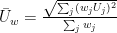
• We are interested in finding the most accurate result, i.e. the result where the relative uncertainty is smallest (i.e. where of a bin is minimized).

The following applies to any particular bin where we want to calculate the average over:

In our bin, we have $N$ datapoints, with scattering cross-section values $I_j$, and associated uncertainties $U_j$. We would like to weigh the data point with the smaller relative uncertainty heavier than the datapoint with the larger uncertainty.

Unweighted, we get for the average intensity and propagated uncertainty :
, and

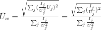
For averages and uncertainties of values weighted with , these become:
, and

In addition to the propagated uncertainty, we can also determine the standard error on the mean. For an unweighted system, this is defined via the standard deviation , with the standard error on the mean then defined as:

The standard error on the mean for weighted data, however, is not quite so easy. From this source, we obtain the following definition for converting a weighted standard deviation to an estimate for the standard error on the mean:

, with
, and

This does require the weighted standard deviation to be known, but fortunately the Python “statsmodels” package is available containing weighted population statistics methods in “statsmodels.stats.weightstats.DescrStatsW”.

We have the following options for weights (or at least the ones I considered to be potentially relevant):

1. no weighting
2. inverse error
3. inverse relative error
4. squared inverse relative error
5. inverse relative squared error

We find the best option by checking which of these weightings gives us the smallest relative propagated uncertainty on the mean (as before: where is smallest). After choosing a set of twelve random values for intensity and uncertainty, we get the following results:

Weighting option 0: average = 0.6183 +/- 0.1816, relative error: 0.2938
Weighting option 1: average = 0.6303 +/- 0.1148, relative error: 0.1821
Weighting option 2: average = 0.7678 +/- 0.1204, relative error: 0.1569
Weighting option 3: average = 0.8741 +/- 0.1136, relative error: 0.1300
Weighting option 4: average = 0.8133 +/- 0.1046, relative error: 0.1286

Ridiculous precision notwithstanding, we do see that option 4 gives us the smallest propagated uncertainty. The mystery here is that I can’t quite figure out why it should be this one. Entering the weighting in the equations for mean and uncertainty, we get:

That means that the mean weighted intensity and uncertainty are defined as:
, and

But even from filling in the equations, No further insight is gained on why this choice of weighting would be the best.

On the positive side, it does work. Check out the merge of some test data in the figure of this post, and see the difference between the averaging done without and with consideration of uncertainty-based weights.

This data has some issues, with a slight upswing at high Q of every dataset (an issue we’re tracing at the moment), and thus serves well to prove the value: the datapoints with better statistics should be weighted more heavily in the averaging procedure than the upswung datapoints with poor uncertainties.

Also plotted are several uncertainty estimators for the intensity; the infamous 1% of intensity, the weighted standard error on the mean, and the propagated uncertainty from the original datasets. For the combined uncertainty, the largest of these three is chosen (per datapoint). It is interesting that the propagated uncertainties are rarely ever as large as the weighted standard error on the mean, and that the 1% limit is rarely reached as well. Nevertheless, having more estimates gives you more of a choice. It is nice to see too, that the few outliers on the binned data do have appropriately large uncertainties, and will, therefore, not be weighted heavily in the fitting procedure.

Also, we see that the propagated uncertainty as well as the standard error on the mean is lower for the uncertainty-weighted averaged data, proving the point that the weighting has a beneficial effect on the quality of your final data.

Lastly, just take a look at that Q- and intensity range we get with our MAUS. That’s 3 decades in Q, and nearly eight in scattering cross-section. We haven’t even tried to go to high Q yet, nor have we installed the USAXS either. Plenty of room, therefore, for expansion!