How to fit a scattering pattern part 2: Some simple fits

Note: Part one of this three- or four-part series can be found here. Additionally, my topical review paper on SAXS data collection and correction which also lightly discusses data fitting is available open access here.

After the initial “scoping out” of a collected scattering pattern, it is time to try to see what can be done in terms of fitting in step 2. Here, we are trying to see if parts of the scattering pattern might be described by some basic scattering functions. 

From Step 1, you should have:

• Complementary information on your structure such as an electron micrograph, X-ray absorption data, crystallographic information, or the production process to name but a few. While I did not touch on this much before, do not proceed without such information as you need to be able to substantiate the structural assumptions that go into the fitting procedure. If you just start fitting, you will end up with a model that matches the scattering behaviour, but has no basis in the actual nanostructure. From the complementary information you should be able to deduce what kind of scattering entities you have in your sample.
• An idea of the background level. If you do not see a constant background level appear, double-check that the background subtraction has not been overdone. An over-subtraction of the background often occurs when the differences in transmission factor (in the sample and background measurements) have not been taken into account
• An idea about whether or not a constant slope should be taken into account (originating, for example, from inter particle scattering and/or large-scale structures.
• Information on whether or not you should consider a structure factor. This may not always be apparent from the scattering pattern.
• Whether or not there is anything interesting at all in the scattering pattern. If not, consider measuring in a different size range or re-evaluating your sample.

What I did not talk about last time is that the scattering pattern may have a peak as well, usually appearing at the larger q-values. This can be a diffraction peak from a long-period structure. If there is an upswing in your data at the higher q-values, you might be seeing only the tail of such a peak, or you might have performed insufficient subtraction of the background scattering signal.

An idea about the approximate size of the scatterers can also be obtained in some cases. If you see a “hump” in your log-log plot, their radius can be approximated by determining the q-value of the peak, and simply calculating . This should give you a rough idea about what size-range your structures are. As indicated by the tone of the preceding sentences: don’t just publish this figure!

For this fitting explanation, I will be using SASfit from J. Kohlbrecher and I. Breßler, but other programs may be usable as well. I have adapted a real dataset for this explanation, from precipitates in a metallic sample. This dataset can be downloaded from here.

What we are trying to obtain in step 2 of the fitting procedure is an idea what the final model should contain. If we have more than one sample in the series (always a good idea, a blank and some intermediate samples to show evolution), we have to test this model on a few samples of the same series. A single model that is capable of describing the scattering from most samples is much better than a tuned model per sample as it will be much easier to show interrelationships.

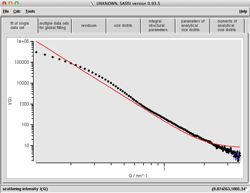
The first goal is to describe the background contributions in the scattering pattern. A quick glance at the data shows a sloped background feature. While there is no clear indication of a flat background, we usually include it anyway. With SASfit, you might need a bit of perseverance and patience, but you’ll get there (in particular, “apply” the proposed parameters first before starting the fit, and only start the fit if the initial configuration intersects the data). The result of this can be seen in Figure 1.

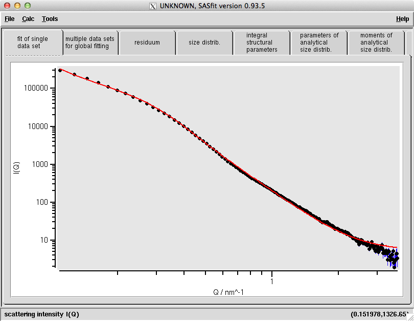
This fit doesn’t look like much, but it’s a start. We can now add a contribution of scattering objects to describe the rest. If you know you have spherical scatterers in your sample, add spheres. Choosing to start simple with spheres conforming to a Gaussian size distribution already fits the scattering pattern quite well (Fig. 2).

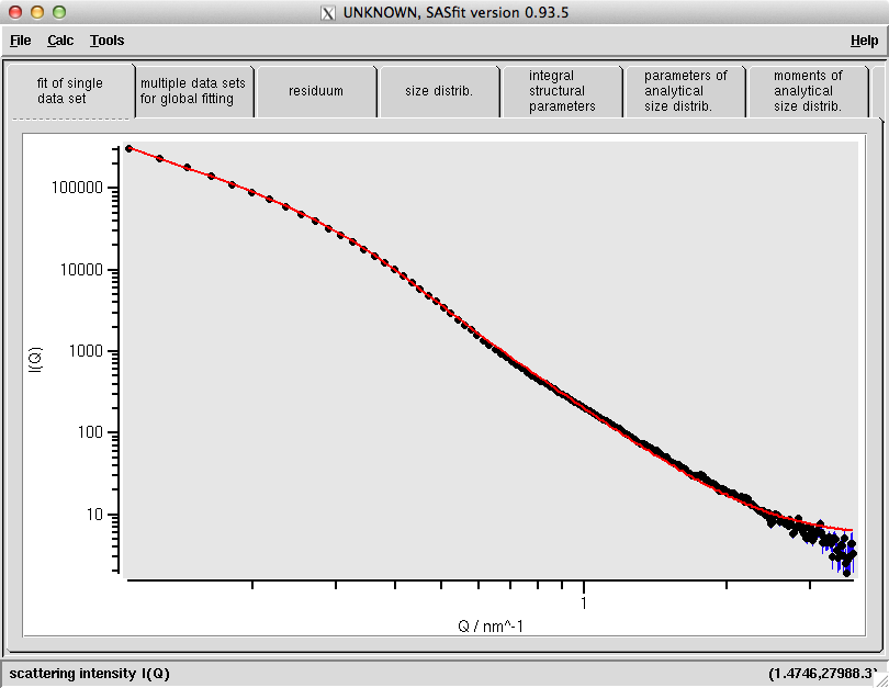
The electron micrograph shows that we have cylinders, not spheres (trust me on this). So selecting long cylinders returns a fit which is very similar (also in terms of reduced chi-square, which is slightly larger than 8 in both cases).  You cannot tell (comparing Fig. 3 with Fig. 2) which is better from the fit itself, which is exactly why the supplementary information is so important: the fit will fit, but the numbers will be wrong!

Given the limitations of the classical analysis methods, this is where I would stop in this fit. One should try out a few more distribution shapes (log-normal, lorentzian) to get a slightly better fit, but adding contributions would be unwise. Adding contributions would destabilise the fit quite quickly, and might make the model justification exponentially harder. Also, do not “hunt” for a fitting model that describes the data best, and then try to argue why that model should be correct. Your model choice should be firmly grounded in other evidence.

One other thing you can do to try to fit your data, is to apply Greg Beaucage’s unified fit function. This function is a combination of two scattering simplifications: a Guinier-like behaviour and a Porod-like relationship. While this function is based on a rather severe set of assumptions (detailed in his publications), it has booked several successes in describing multi-scale scattering effects. This function might be able to provide some insight into the size range of the structures under investigation.

While this is only a straightforward example, there are an enormous amount of alternative fitting functions available for the strangest scatterers. Chances are that one has been developed for your system as well over the past 80 years of scattering, so please search for the most appropriate function and do not automatically head for the Porod, Guinier, Debye-Anderson-Brumberger or other heavily approximated functions. And always verify that the answer you get from the fitting is realistic.

For more hints and tips on data fitting, please check out the last section of my review paper!

 

[fitting data (asterisk indicates inclusion in optimisation function):

Long cylinder model (L=70, eta=0.1) w/gaussian distribution (N=1.6*, s=2.64*, X0=3.42)  and added background contribution (c0=5.35, c1=0, c4=16.6*, alpha=4). Reduced chi-squared: ~8.6

Sphere model (eta=0.1) w/gaussian distribution (N=8.15*, s=3.26*, X0=3.38) and added background contribution (c0=5.28, c1=0, c4=29.6*, alpha=4). Reduced chi-squared: ~8.5]