

It has been a very quiet four months (since this post) on the Bonse Hart front, as the generator was out of order (yes, again, and again). However, on one of the last days of 2013, something stirred in the lab, unsettled some dust and replaced the broken part. While I am not quite sure if the cause has been fixed or just the symptoms, the end result is that I can run the generator again at (at least) 10% power without things blowing up at me.
Over the last few weeks, I have therefore spent a lot of time in the labs to try to continue where I left off: characterising and improving the measurement capabilities of the instrument. When last we met, there were 100 k counts per second in the direct beam over a background of 10 counts per second. This background needed improving.

With the generator (Figure 1) at 10% power, the direct beam intensity through the second crystal is no better than about thirty kilocounts per second. Despite this low power, the background was about 20 counts per second in this set-up. The first attempt at reducing this was to introduce some shielding on the detection surface: to mask everything but a small area around the crystalline reflection. Some scrap metal and a slit I took off of another instrument took care of this, and reduced the background signal to about 7 counts per second. Still a bit high.

Looking at the pulses coming in on the oscilloscope (I really have to get a new one of those some day, as mine is about 40 years old and regularly goes on the fritz), I noticed that the background pulses coming in weren’t all that nice at all. So I decided to adjust the pulse amplifier and narrow down the single channel analyser (SCA, see Figure 2). The SCA is a simple circuit that checks the height of the pulse that comes from the amplifier (and which should be roughly proportional to the photon energy on the scintillator detector): pulses of the right energy of around molybdenum k-alpha should be passed through, the rest rejected. A better adjustment of this system reduced the background to about 1 count per second. So far so good!
Playing around placing pinholes in odd locations, I finally managed to reduce the background a little bit more (by about 0.4 count per second) by placing another slit between the two crystals (wider than the direct beam). I didn’t think this would work, and that it would create a higher parasitic scattering background, but apparently it’s no problem to do this. So one more lesson learnt: play around and don’t rely on instinct!
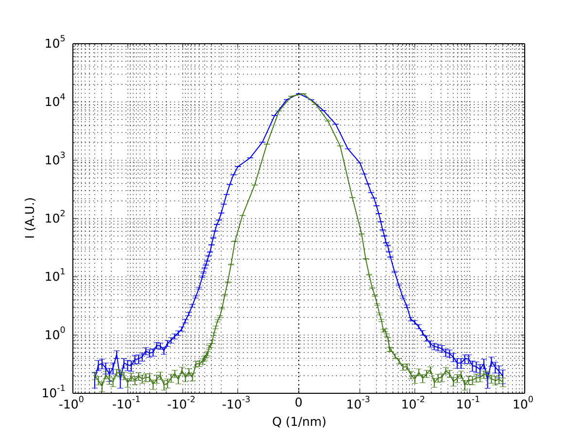
After reprogramming the measurement points to assume a mostly logarithmic spacing except for directly around the beam position, I measured a background and a sample. Correcting both for the detector dark current (now at 0.134 counts per second with the shutter closed) and correcting the background for the sample transmission, I managed to get a very promising measurement (Figure 3).
Apparently, we have a decent signal-to-background ratio between 0.001 < q (1/nm) < 0.01. I’m not so confident about the datapoints beyond that. There appears to be something valid, but it is a rather small signal to distinguish. More to follow on this aspect.
So what’s next? Well, I have to try to get more photons through, and I’d like to reduce the background a bit more if possible. Secondly, I need to implement a small interpolation program so I can subtract the background signal from the scattering signal. Lastly, I’ll have to see if a Lake desmearing method can be programmed into python. If not, Jan Ilavsky’s programs are just ’round the bend!
Leave a Reply