

Last week, I talked about how to determine whether a flatfield correction was necessary. Data from a Bruker Hi-Star detector was shown to have very large local sensitivity deviations in the 2D detector image (of +/- 50%), and would therefore need a flatfield correction. So how to get one?
The normal method for getting the flatfield of a Hi-Star detector is to use a radioactive (iron) sample to evenly illuminate the detector. This method has two issues. Firstly, you’d be measuring for a bloody age to get any sort of per-pixel precision with the current low activity of the radioactive samples sold. Secondly, for our instrument it means changing the bias settings of the detector, which may change the flatfield response.
Another way to get a flatfield correction is to compare the measured pattern of a sample with the pattern it is supposed to show. For most samples we do not know what the pattern is supposed to be, but there are a few exceptions.
One such exception is a glassy carbon sample for absolute intensity calibration (from friends at the APS, for example). These samples come with their own calibrated dataset, which tells you exactly how it’s supposed to scatter. Last week, I tried to get this working in time for the post, but didn’t manage. It’s finished now, which means I can show you how much it would matter.
Firstly, let’s compare the integrated (measured) pattern to the external (calibrated) dataset provided with the sample. For this, we now have a “CurveComparator” module in the imp2 data reduction methods. As many corrections as possible are performed on the data, to make it the best possible representation of the final curve. The comparison is shown in Figure 1.
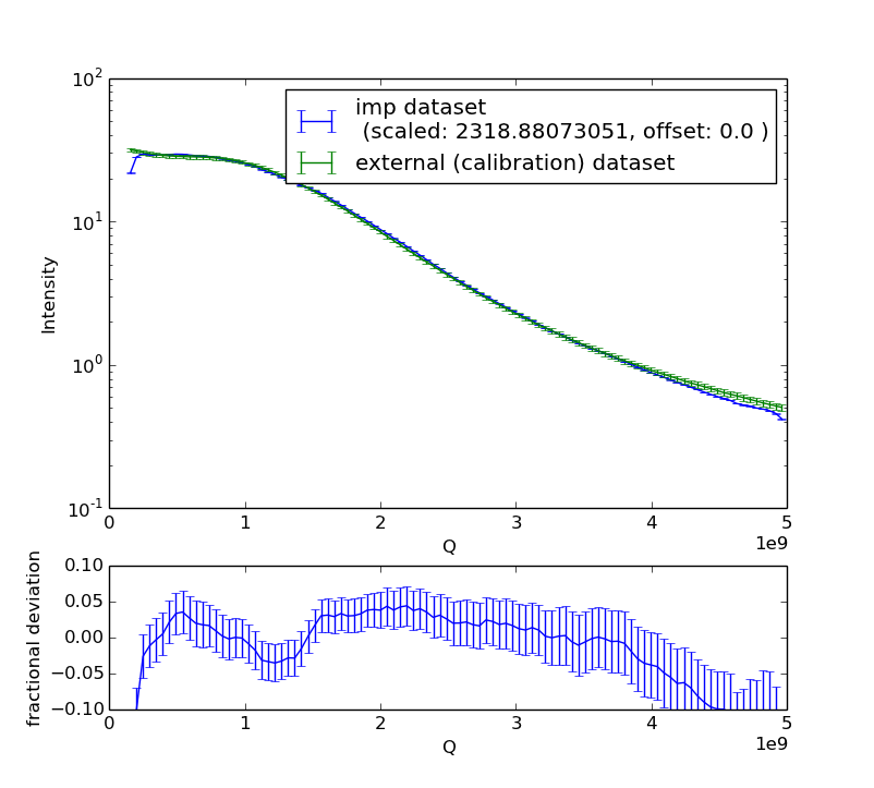
Now, the uncertainties look rather large on the fractional deviation. This is because the error bars shown are the propagated uncertainties of both the integrated data and the external dataset. I know that the uncertainties on the external dataset are a bit overestimated. Nevertheless, the data shows systematic deviations from the calibrated data, with differences in the low-Q region of the integrated dataset of about 5%, and 10% at high-Q. The results from fitting a dataset measured on this instrument, therefore, will be just as rubbish as the data that went into the fit. We need to do the flatfield correction to get data to a more reasonable accuracy.
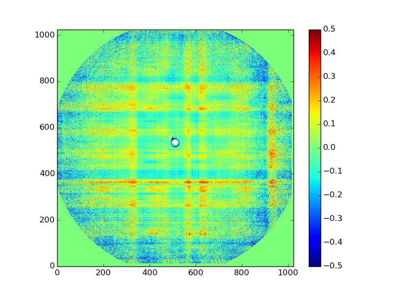
We can determine the flatfield of the data by comparing the local reading on the 2D image of the detector with the (external) calibration data (Figure 2). This looks a lot like the image of last week, but this is the flatfield that should be used as this one will correct for the deviations in the integrated data. This one also shows a decrease in sensitivity directly around the beamstop, which is probably an effect of partial shadowing of the scattered radiation by the beamstop and the convolution of the detected pattern with the point spread function of the detector. This region, if used, should be considered suspect at best.
Of course, you can reduce many of these issues by buying a fancy new detector, but where’s the fun in that?
Leave a Reply