

See the previous posts in this series here: Part 1, Part 2 and Part 3
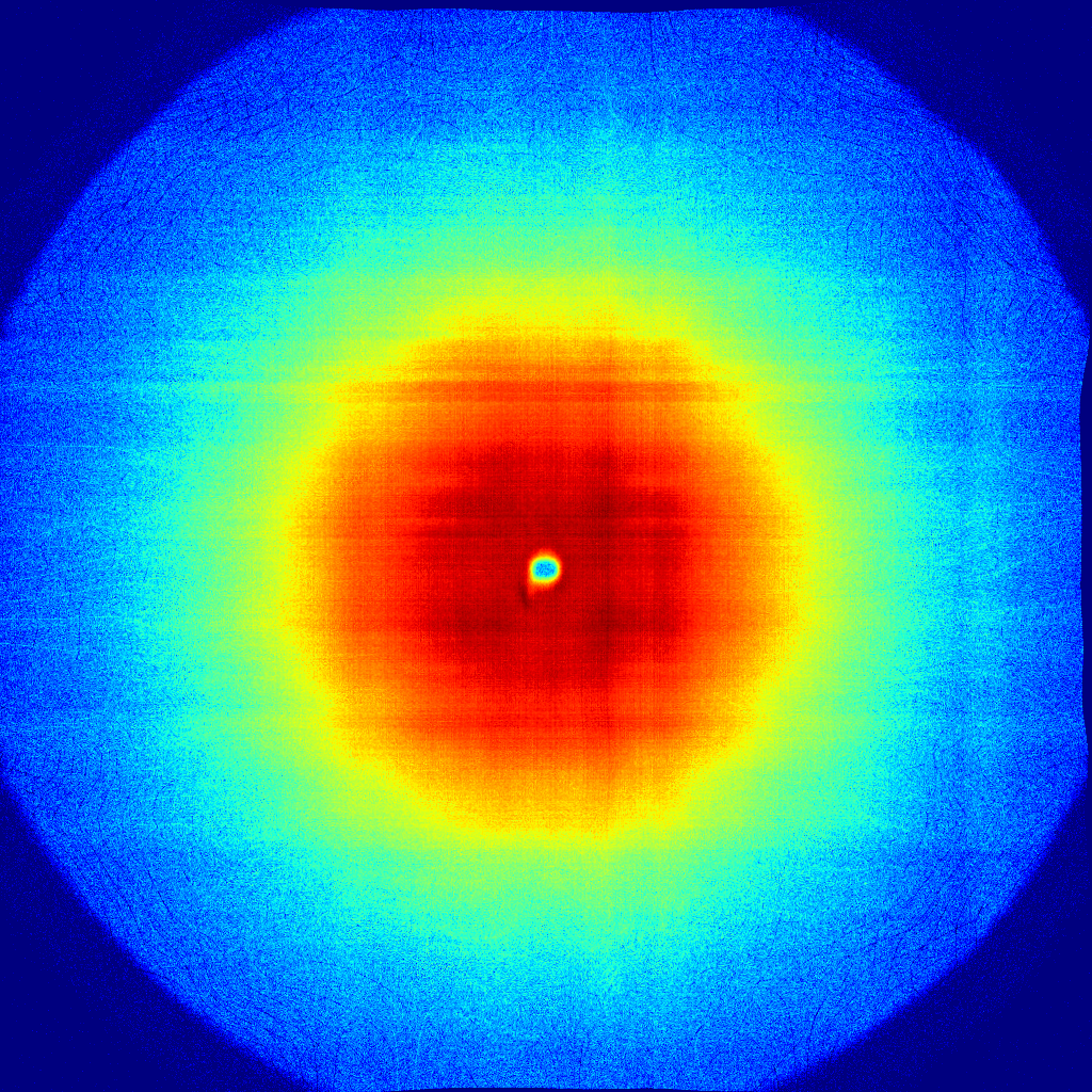
Very recently, Bruker upgraded their SAXS instrument in our building. This is a typical 3-pinhole 2D SAXS system that was largely designed by J. S. Pedersen in Aarhus a decade or so ago. This particular version was at NIMS in the Quantum Beam Unit / Neutron Scattering Group, and was using chromium radiation (a very low energy radiation). Now that its source has been upgraded to my favourite molybdenum type (a high energy radiation), it is time to check all of its corrections once more, starting with the flatfield.As we now have an rather high flux from the instrument, detector inaccuracies show up a bit more clearly than they did in the past. A glassy carbon measurement, therefore, shows clear trouble on the flatfield-front: clear non-uniformity in the detected signal (Figure 1).
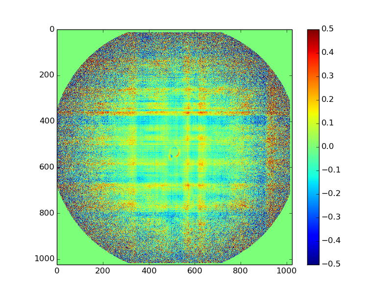
Last week, I updated the new data reduction methods with a tool for showing these deviations. It is based on the previously discussed methods for flatfield generation, where we compare the detected image with that of a known isotropic scatterer. In this case, the detector image was azimuthally integrated to form the “known” pattern (which is not a perfect solution, but it will do for a first look), and the local response was compared to this pattern (Figure 2).
As the results show, the Bruker HiStar wire detector is actually pretty bad: there are local positive and negative deviations of up to 50%! This will not do. Given these large deviations, however, we cannot be sure that the azimuthal average actually gives us the correct values (as all or most of the pixels on the azimuthal averaging circle can, for example, return too high values). Fortunately, the glassy carbon sample we used comes complete with its own calibrated datacurve (thanks to Jan and his team at APS).
Using this, we can get a better picture of how far off the measured intensities really are, and what effect a flatfield correction would have on the azimuthally integrated curve from real samples. This is a task which is not yet completed (and I could not get it working in the hour or so before this post has to go live), so I must delay the conclusion to this story until such a time when it is.
But as an intermediate conclusion: yes, a flatfield correction is absolutely essential for this (and similar) detectors.
As usual, leaving comments is highly appreciated!
Leave a Reply