

We left off this issue a few weeks ago after discussing the variations between the datasets. However, we did not evaluate how variations in the data affects the final morphological parameters. Let’s do that now.To evaluate this, we fired up McSAS and let it analyse each collected scattering pattern. In order to avoid artifacts, the radius range was adapted to match the limits imposed by the data for every pattern.
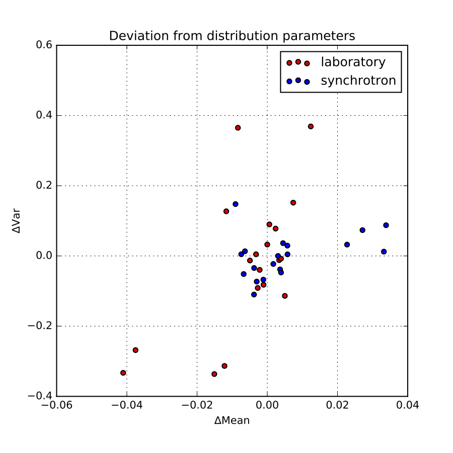
Each resulting distribution was quantified in terms of the distribution moments, in particular the mean and the variance. We can determine the median mean value, and the median variance, and plot the fractional deviations from those. This is shown in Figure 1, where an additional separation has been made between synchrotron and laboratory instruments. The horizontal axis signifies the deviation from the mean, and the vertical axis plots the deviation from the variance.
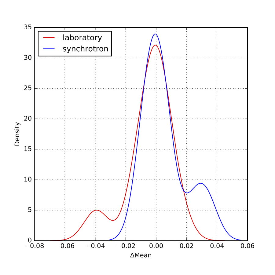
As can be estimated from that figure, there are a few outliers, but most data appears within about +/- 1% of the mean, and +/- 10% of the width. At first glance, there appears to be no obvious difference between synchrotron and laboratory instruments. We can, however, plot the distribution of deviations as a kernel density estimate plot. This is shown for the means in Figure 2, and for the widths in Figure 3.

These plots show that the distribution of values for the means are indeed independent of whether it was measured on a laboratory or on a synchrotron. The widths, however, do show a wider spread for laboratory instruments than for synchrotron instruments. When calculated numerically over the entire set, one standard deviation of the mean is about 1.6%, and of the variance about 9%. Quite good for this technique, I’d say!

Finally, each laboratory was sent a pair of samples, and was requested to measure both of them. These samples were identical (which I can say now that the deadline has passed). These pairs allow us to estimate the intra-instrument precision as well, by quantifying the distance between the values of each pair.
These distances are shown in Figure 4, which shows that the intra-instrument precision is (as expected) better than the inter-instrument precision. However, here we are falling within the uncertainty of determination using McSAS. Therefore, we’ll switch to another program (with added assumptions) to try and quantify this a little better.
We are now working on the publication of these results. A very big thanks to all the laboratories who have graciously participated in this project, without whose efforts we would not have been able to determine the precision of SAXS. The anonymized, rebinned data will be made available under a creative-commons license after publication to allow further evaluation by you. As always, comments can be left in the comment section below!
Nice job! It would beneficial to the labs that have generated outlier values if you tell them (there are just very few, actually!). They might then improve their set-up.
Really cool work Brian. Congratulations on collecting such a conclusive dataset. Seems as if SAXS is indeed a good method to measure small things ;)
Hi Javier,
I will be sending out personalized charts next week with the location of the person’s lab indicated on the chart. That way everyone can know where they are (but no-one knows the position of others unless the others have made it public). I already know of one participant who was able to use the data to improve their lab.
Cheers,
Brian.
Thanks, Tilman!
Very nice, thanks a lot for the effort you put in. It is good to see that SAXS seems to agree with itself rather well.
Thank you very much, Martha. You’ve hit the nail on the head, this round robin shows that SAXS agrees with itself quite well, but makes no claim to the accuracy of the sizes found. Perhaps everyone is off by a nm or two!
That’s a very valid point. Brian, do you have plans to extend it to some real-space verification like TEM or something like that to adress this issue as well?
We’re working on it!