Applying five estimators for uncertainty in Q

2016-10-26 Brian Pauw Blog posts 7

In order to get any sense of the uncertainty on our size determinations, we need to find out what the uncertainty of the q-vector is. In the “Everything SAXS”-paper, I mentioned that it is possible to estimate (at least) five of these. We have now done this for our own Kratky instrument…

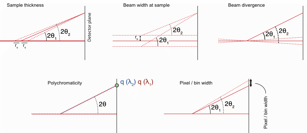
The (updated) drawings depicting the uncertainty sources are given in Figure 1. To evaluate the worst-case magnitude of these (i.e. calculating the extrema of the uncertainties), we need to know the details of the geometry of the instrument.

The geometry of the instrument

The Kratky camera employed for our measurements has an approximate (fixed) sample-to-detector distance $l_{sd}$ of 307 mm and a sample radius $r_s$ of 1 mm. The pixel size on the Dectris Mythen detector attached to our Kratky camera is 50 $\mu$ m, with no point-spread function. The X-ray spectrum reflected by the multilayer optics largely consists of Copper k $_{\alpha 1}$ and k $_{\alpha 2}$ radiation, whose mixture gives us an weighted apparent wavelength of 0.1542(2) nm. When we assume perpendicularity of the detector with the point of normal incidence at the beam center, the $q_{pixel}= 4\pi / \lambda \sin(\theta_\mathrm{pixel}) = 6.64\times 10^{-3}$ 1/nm. The useful data in these experiments has been defined to start at $q = 0.1$ 1/nm. We have been informed that our instrument optics has a focal length of 500 mm towards the beamstop, which corresponds with a convergence angle of 0.13 degrees.

The finite sample thickness contribution

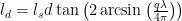
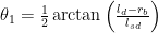
We can determine the sample thickness-induced uncertainty in q, $\Delta q$ , using:
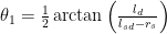
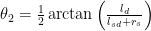
$\Delta q = \frac{4 \pi}{\lambda} \left\{ \sin \theta_1 - sin \theta_2 \right\}$ where
$\theta_1 = \frac{1}{2} \arctan\left( \frac{l_d}{l_{sd} - r_s}\right)$ and
$\theta_2 = \frac{1}{2} \arctan\left( \frac{l_d}{l_{sd} + r_s} \right)$

where $l_d$ is the distance on the detector from beam center to the point of interest.

We calculate $l_d$ from our reference $q$ vector using:
$l_d = l_sd \tan \left( 2 \arcsin \left( \frac{q \lambda}{4 \pi} \right) \right)$

(result in Figure 2 below)

The finite beam width contribution

This is the issue of the beam not being infinitely thin. That means that scattering originates from multiple heights in the sample. This is calculated virtually identically to the above correction, except that we are adding the radius of the beam $r_b$ to $l_d$ instead of $l_sd$ :

$\theta_1 = \frac{1}{2} \arctan\left( \frac{l_d - r_b}{l_{sd}}\right)$ and
$\theta_2 = \frac{1}{2} \arctan\left( \frac{l_d + r_b}{l_{sd}} \right)$

The resulting $\Delta q$ due to beam finite beam height is constant over the q-range with a magnitude of 0.04 1/nm. As expected, this uncertainty is largest the closer to the beam you get, where it assumes about 40 % of the q value. This contribution rapidly increases towards smaller q, however, so it is worth keeping it in mind for future checks.

The uncertainties originating from pixel or datapoint widths

The finite pixel- or datapoint size gives us a width in $q$ that can affect the resolution of the smaller scattering vectors.

We distinguish between pixels and datapoints, as the data in multiple pixels may have ended up in a single datapoint during the averaging or re-binning procedure. Geometrically, we have a lower limit of the precision defined by the pixel width. As given in the geometry section, this means that we have an uncertainty of no less than $6.6\times 10^{-3}$ 1/nm at $q=0.1$ , or 7 %. For the pixels higher up in q, this uncertainty will gradually decrease.

The minimum q-point distance in our dataset is the same at $latex q = 0.1$, implying that we have not lost precision through the re-binning procedure for the first datapoint. For the later datapoints, however, more and more pixels have been grouped together to form a single datapoint.

Along the Q-vector of our measurement, the relative ∆q/q span of each binned datapoint can be determined, and plotted for a typical measurement in Figure 2.

The uncertainty originating from the beam divergence

The beam divergence is dictated by the collimation as well as the optics. In our instrument, the beam is focused on the beamstop, and using that information together with the width of the beam at the sample position, allows us to estimate the effect of divergence. This calculation can be done quite similar to the estimates from before, but where we add the divergence angle from the straight beam $\theta_d$ to the angles:

$\theta_1 = \frac{1}{2} \arctan\left( \frac{l_d}{l_{sd}}\right) + \theta_d$ and
$\theta_2 = \frac{1}{2} \arctan\left( \frac{l_d}{l_{sd}} \right) - \theta_d$
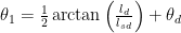
where
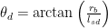
$\theta_d = \arctan \left(\frac{r_b }{ l_{sd}}\right)$ , or known from the optics manufacturer:

$\theta_d = \frac{1}{2} 0.13 ^\circ$

Calculated thus, the $\Delta q$ due to beam divergence is constant over the q-range with a magnitude of 0.18 1/nm. This is very large, and as we will see in the result, the largest contribution by far.

The polychromaticity contribution

The emission lines passed through by the mirror contain both the $k_{\alpha, 1}$ as well as the $k_{\alpha, 2}$ energies (actually, the mirror also allows through higher order energies from brehmsstrahlung, but that is another problem for another time). These two energies bring about a small change in wavelength, and therefore $q$ -vector. It is very small, but we include it here for completeness.

We estimate the thereby induced uncertainty in q, $\Delta q$ , using:
$\Delta q = \left( \frac{4 \pi}{\lambda_1} - \frac{4 \pi}{\lambda_2} \right) sin \theta$ where
$\theta = \arcsin \left( \frac{q \lambda}{4 \pi} \right)$

(shown in Figure 2)

The final score and effect

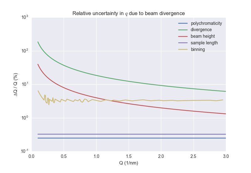
**Figure 2:** Relative contribution of each uncertainty contributor to q.

Plotting the relative uncertainties in Figure 2 shows us that the divergence, or in this case the convergence, has a dramatic effect on the uncertainty in q. This is the extreme estimate of the uncertainty, but it does reinforce my hesitation when it comes to the benefit of focusing optics in small-angle scattering. The second interesting bit is the bin width contribution. We see here that the logarithmic binning scheme we employ is actually quite nice in this respect, keeping the relative uncertainty contribution nicely constant (we talked about that binning before, here). The only other significant contributor to the uncertainty is the beam height, which tells us that for low-q details, the beam must be restricted in dimensions.

The effect on the scattering pattern

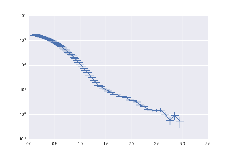
The effect of the largest Q uncertainty contributor, the convergence, shown as horizontal error bars to the curve.

The effect of the largest uncertainty estimator, the convergence, on the scattering pattern is shown in Figure 3 for an example curve. This shows a pretty significant contribution, and raises some questions in my mind about its validity in practice. We do have a plethora of arguments (excuses) ready on why it wouldn’t be like this, for example:

The beam convergence angle is weighted towards the horizontal, and so it isn’t all that bad… probably.
We should be showing 1SD confidence intervals instead of the extrema. This would reduce the visual emphasis, but not the underlying issue.
We didn’t take into account the single-sided limitation to the divergence potentially introduced by the Kratky collimation.

The worst of the arguments (in terms of traceability) is that we perform the rather black art of desmearing on the data once received from the instrument. That means that some of the broadening in Q has been counteracted at the penalty of higher uncertainties in the intensity. The thus-introduced reduction in our Q uncertainty is very difficult to assess. We are therefore in this case limited to using practical estimators for the uncertainties, at least in the case of the Kratky-class instruments (something like this?).

If you have the time, I would very much like to see the estimates of these contributors for your own instruments. A Jupyter Notebook worksheet is available on request (i.e. once someone requests it, I’ll have to take the time to clean mine up, pepper it with clarifying comments, and send it).

Fred
2016-10-27 at 21:45

Nice post, Brian !
Correct me if I am wrong, but I think what you describe here is not an “uncertainty” on q, but rather what is usually called “q resolution”, especially in SANS where it can be very prominent. It is not an “error” on the q position of the data point, it rather means that this particular data point probes a q-range which is described by this resolution. In other terms, you “simply” describe the amount of smearing of your instrument. Since you then go on and desmear it, I am not sure what you end up with…
Brian Pauw
2016-10-28 at 15:49

Hi Fred,

Indeed, these are the “q resolution”-smearing contributions. I should have perhaps named this more appropriately. I think that when we are counting per photon, though, it is an uncertainty: any photon can arrive with a Q vector anywhere (albeit with a weighted probability) within the bounds of the examples above.

In the Anton Paar-implemented desmearing procedure, we mainly correct for the finite beam width, which is a contribution I did not describe in the article above as it is specific to the Kratky-type instrument. However, this desmearing procedure does not explicitly correct for any of the abovementioned contributions, e.g. the divergence or beam height at the sample. Whether that is coincidentally corrected for during the beam width desmearing procedure is not something I know.

The next part (maybe next week or otherwise the week after) will have some practical estimators and calibration exercises. I hope that’ll answer some of your questions!
Fred
2016-10-28 at 16:53

Well, granted, you are counting photons, but you are integrating a certain number of photons, so you are integrating within the q-distribution. It could be considered as an “error” if you were considering a single photon q. But what you are doing is integrating a certain number of photons, and plotting their number as a function of their corresponding q (which have a certain distribution).
Brian Pauw
2016-10-31 at 08:59

Yes, so what we call “smearing” is essentially the observation of the uncertainty distribution in q. The approximations in this blog post allow you to assess how large that smearing could (maximally) be.
Andrew Jackson
2016-11-16 at 15:53

Indeed in SANS, at least 4 of the estimators presented here are folded into the resolution function (thickness not normally included). The data are then preferably not desmeared, but a model for the data is smeared with the resolution function (since the resolution smearing involves a genuine loss of information and the reverse is a many-to-one proposition, though in mild cases it is an acceptable approximation).

For other readers, some relevant papers might be :

Mildner, D. (2005). Resolution of small-angle neutron scattering with a refractive focusing optic. Journal of Applied Crystallography.
Barker, J., & PEDERSEN, J. S. (1995). Instrumental Smearing Effects in Radially Symmetrical Small-Angle Neutron-Scattering by Numerical and Analytical Methods. Journal of Applied Crystallography, 28, 105–114.
Harris, P., Lebech, B., & PEDERSEN, J. S. (1995). The Three-Dimensional Resolution Function for Small-Angle Scattering and Laue Geometries. Journal of Applied Crystallography, 28(2), 209–222. http://doi.org/10.1107/S0021889894010617
SINGH, M. A., GHOSH, S. S., & SHANNON, R. F. (1993). A Direct Method of Beam-Height Correction in Small-Angle X-Ray-Scattering. Journal of Applied Crystallography, 26, 787–794.
Mildner, D. F. R., & Carpenter, J. M. (1984). Optimization of the Experimental Resolution for Small-Angle Scattering. Journal of Applied Crystallography, 17(AUG), 249–256.
LAKE, J. A. (1967). An Iterative Method of Slit-Correcting Small Angle X-Ray Data. Acta Crystallographica, 23, 191–194.
Andrew Jackson
2016-11-16 at 15:56

I would also add that when operating a neutron instrument in “event mode” – i.e. recording every neutron detection event – figuring out the resolution function for a given Q bin is an important part of the data processing procedure. In many cases the function can be represented by a simple gaussian, but one can generate interesting cases where that is not true.

This is one of the reasons for the extended capabilities to record uncertainties that we put into the NxCansas data format.

What to do with Q? – Looking At Nothing

This site uses Akismet to reduce spam. Learn how your comment data is processed.

Looking At Nothing

A SA(X)S Weblog