

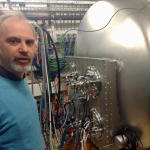
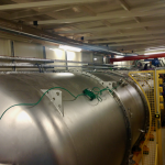
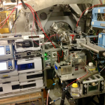
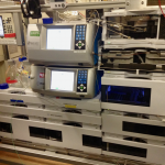
Last week, I’ve had the pleasure of visiting France for three days, seeing Olivier Taché and friends at CEA, Javier Péréz and co. at Soleil and Marianne Impéror and her group at l’Université Paris Sud. Here’s what we did…
First, let’s start off with some pictures to give you an idea of the sights:
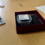


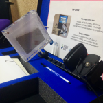

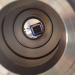
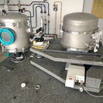
At the CEA, we played around with their new Xeuss instrument. My main interest was finding out if the collimation settings might affect the coherence, and therefore the scattering pattern (following this story). I had brought two samples, disc-shaped cellulose pellets, one pure cellulose, and the second cellulose plus a porous carbon sample from Zoë.
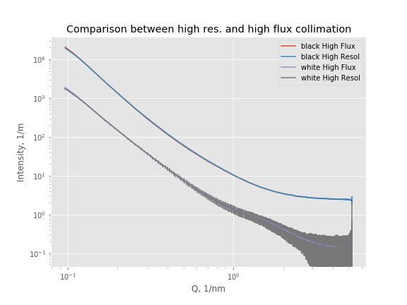
We corrected the data for the, darkcurrent, transmission, flux and background using Olivier’s PySAXS procedures. At the moment, this only does linear binning, but that’s good enough for what we are trying to do. We look in Figure 1 at the data from the two samples with the two different collimation settings, “high flux”: 1.2 x 0.8 mm (v x h), or “high resolution”: 0.6 x 0.5 mm (v x h). The direct comparison shows no difference, except very close to the beamstop, which is to be expected due to smearing and shadowing effects. Case closed? Not quite.
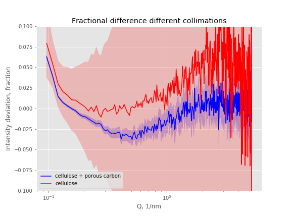
A double-logarithmic plot hides all kinds of effects. We can do a better comparison, by looking at the fractional difference between the scattering patterns (Figure 2). Doing that, we see that there is a significant and systematic deviation in the data from different collimations, on the order of a few percent. This difference is consistent between the two samples.
One mystery remains about its shape, however. I have no idea why the curve is S-shaped. Further experiments will follow in the near future to shed more light and X-rays on this.
Now you may think I’m (dutch:) “ant-fucking” about these quite tiny differences. But when I get complaints about my habit of constraining the uncertainties to be no less than 1%, I feel the need to do these tests. They show that data accuracy in SAXS isn’t quite as good as we may intuitively think, and I hope I can demonstrate this.
Did you try measuring @ two different distances in the same collimation, such that the ratio of the respective coherent lengths takes the same values as in the high flux vs. high resolution measurement ? If so, do you get the same S shape curves ?
Alas, we did not have time to change the sample-to-detector distances. I also have no idea what length should be chosen then for the second measurement, to keep the ratio identical.
On a pin-hole instrument this should be easier right ? then the ratio of the two distances should match the one of the pinhole openings.