

A while ago on Twitter, there was a question doing the rounds about how much synchrotrons and lab sources really differ in flux. While synchrotrons generally are interested in figuring that out (since it’s their selling point), information on laboratories is a little harder (but not impossible) to find…
Literature comparison
In published information on beamlines (on their sites as well as in papers), we find stated fluxes of:
- 5e12 ph/s (Kirby-2016), beam size 130 x 250 µm FWHM, 12 keV, Australian synchrotron SAXS/WAXS. That translates to 1.54e14 ph/s/mm^2
- ESRF’s flagship (or battleship) SAXS beamline ID02 states a flux on the order of 1e14 ph/s over a beam of 200 x 400 µm at 12.4 keV. That translates to 1.25e15 ph/s/mm^2
- Diamond I22 gives a flux of 6e12 with a beam of 320 x 80 µm at 12.4 keV, translating to 1.95e14 ph/s/mm^2
- MAX-lab’s I711 in 2009 (Knaapila-2009) had a flux of 4e10 in a beam of 0.37 x 0.37 mm, translating to 2.92e11 ph/s/mm^2, although they may since have improved a bit, since their website now claims “>1e11 ph/s”.
- SLS’s cSAXS states 1e12 ph/s at 11.2 keV, using a beam of 0.5 x 0.5 mm, translating to 4e12 ph/s/mm^2.
So all of the beamlines at large synchrotrons seem to be delivering pretty much the same amount of photons, give or take an order of magnitude. How about laboratory instruments?
This information is a bit harder to find. Even papers with very interesting titles like “SAXS instruments with slit collimation: investigation of resolution and flux” (Fritz-2005) contain only relative fluxes. Jan-skov Pedersen has been presenting about flux numbers for his new metaljet-based SAXS, but as far as I can see, that is not published. Here’s what I can find:
- Andras Wacha in 2014 published a value for their CREDO pinhole-SAXS with microfocus source: 165000 ph/s at 8 keV, with a 0.7mm dia. beam at the sample position, translating to 4.3e5 ph/s/mm^2
- Jan-skov Pedersen published in 2004 a value of 1.9e7 ph/s at 8 keV for the total beam in his instrument, although the beam diameter) at the sample position is quite unclear. Assuming 0.5 mm^2, this translates to 9.7e7 ph/s/mm^2. He has since upgraded to a metaljet, which may have increased that by another order of magnitude.
- Linda Brützel in 2016 published a rate of 2.5e6 ph/s in a beam at the sample position of 1.2 x 1.2 mm (microfocus source), which translates to 1.7e6 ph/s/mm^2.
So, some differences there, indicating a difference between labs and synchrotrons of about 1 million. However, we can also go one step further with some practical tests on our instruments.
Practical comparison
Andy Smith at I22 kindly provided us with recent information on his instrument for one of our experiments, with a flux on the sample of about 2.1e12 ph/s in a beam of 0.1 x 0.3 mm, translating to 7e13 ph/s/mm^2. That is well in line with the website claims above.
We did a test on our SAXSess recently, with a tube source and (line) focusing optics. We got 900000 ph/s on an area of approximately 0.75 x 0.2 mm, translating to 6e6 ph/s/mm^2.
During the CEA visit, we also automatically got information on the flux of that microfocus source instrument, which delivered 2.9 ph/s in a beam of 1.2 x 0.8 mm, which is 3e7 ph/s/mm^2.
Conclusion
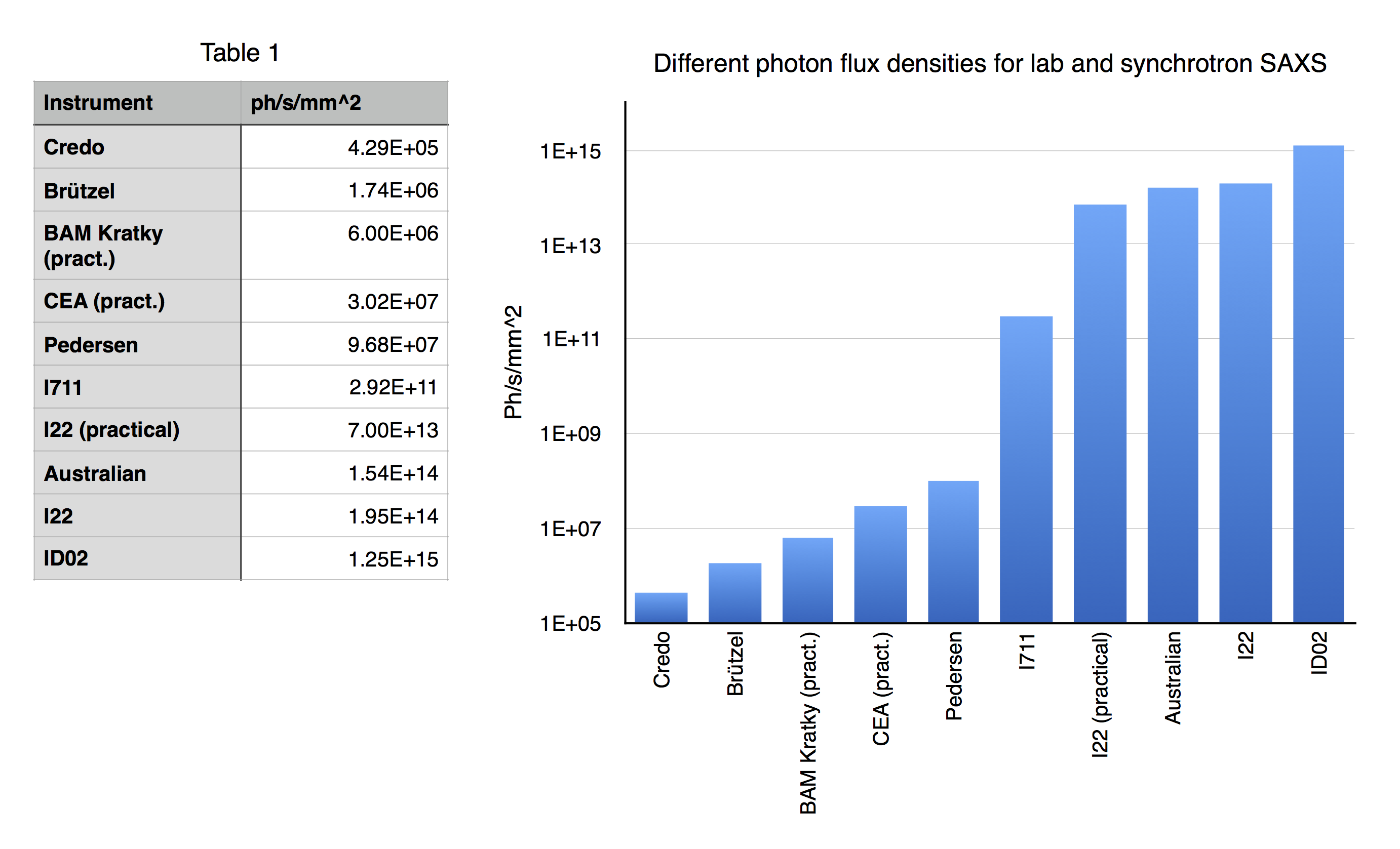
The result is shown in Figure 1, demonstrating there is not just a difference of a million in flux density, but up to a factor of 1e10 between the different instruments! That is an enormous difference. However, one lab instrument in your institute is worth 10 inaccessible synchrotron instruments: If you have the time, and you have a well-optimized lab instrument, you can collect data that rivals the best synchrotrons. Measure overnight, or over the week-end, throughout the year, and take the time to fine-tune those data corrections and sample conditions to get that damn fine quality.
If, however, you find yourself with a (small) sample that changes rapidly over time, then it is good to know you can go faster. Much, much faster: 10 orders of magnitude, to be precise. And that’s when you head to the synchrotron!
Leave a Reply